
yaml2plot: A Python Package for Creating Plots from YAML Specifications


yaml2plot is a powerful yet lightweight Python package for creating interactive Plotly figures from YAML specifications and SPICE .raw files with minimal code. It loads simulation data directly into a simple {signal_name: np.ndarray} dictionary, supports declarative multi-axis plots via YAML configurations, and automatically selects the best renderer for Jupyter, VS Code, or headless environments. With case-insensitive signal lookup and robust multi-strip support, yaml2plot lets you focus on circuit analysis—not plotting boilerplate.
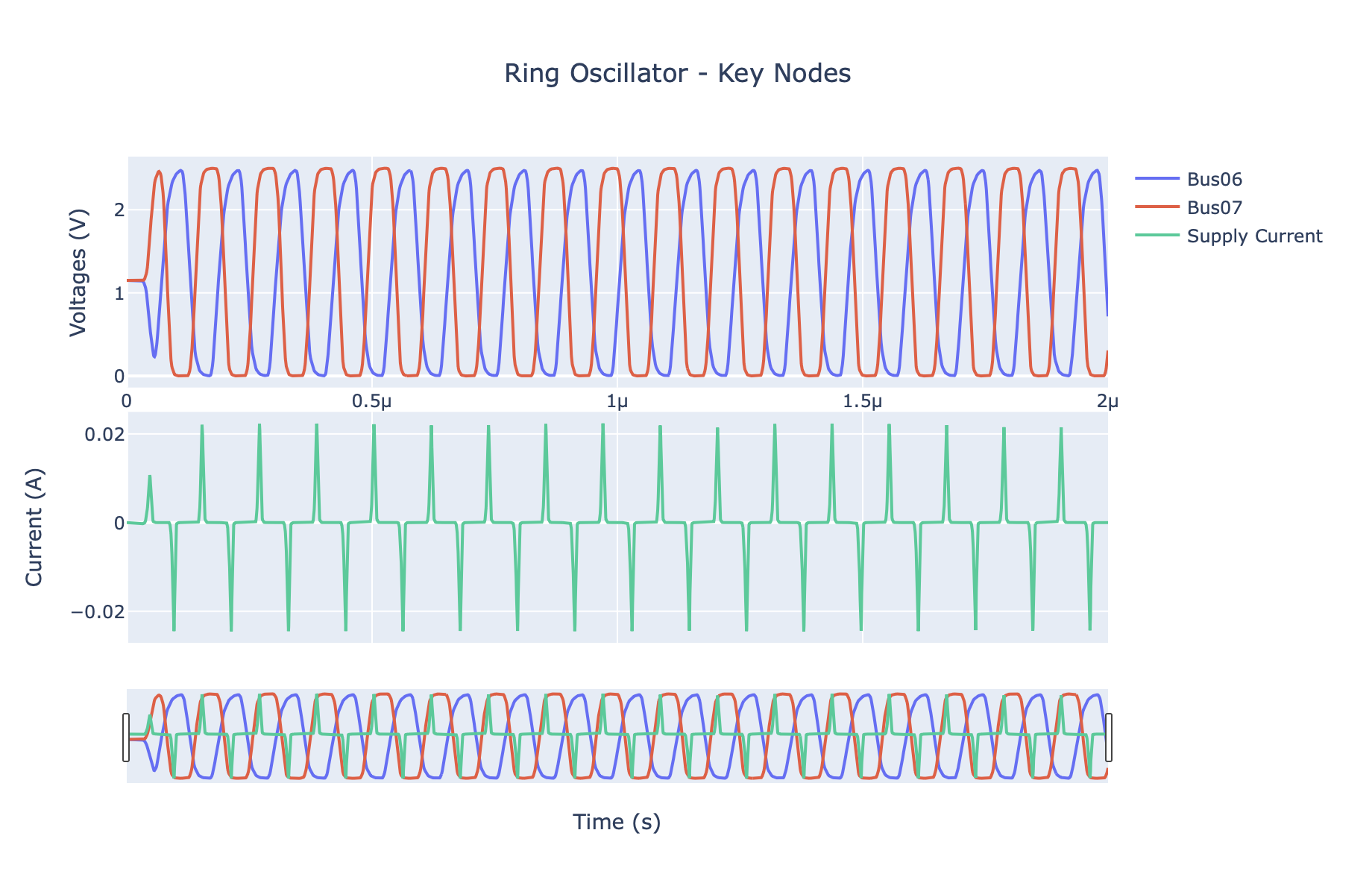
Features
- Interactive Plotly Visualization: Modern, web-based plots with zoom, pan, and hover
- YAML Configuration: Flexible, reusable plotting configurations
- Simple API: Plot waveforms with a single function call
- Command Line Interface: Quick plotting from terminal with
y2p plot - Automatic Environment Detection: Auto-detection and inline plotting for Jupyter Notebooks, render in browser when running in standalone Python scripts.
Quick Start
Installation
pip install yaml2plot
yaml2plot provides two common workflows for visualizing your SPICE simulations:
- Option A: CLI-First – The fastest way to get from a
.rawfile to an interactive plot. Perfect for quick, one-off visualizations. - Option B: Python API – The most flexible approach. Ideal for scripting, custom data processing, and embedding plots in notebooks or reports.
Option A: CLI-First Workflow
Get from a raw file to a plot in three steps using the y2p command-line tool.
Step 1: Generate a Plot Specification
Use y2p init to create a template spec.yaml file from your simulation output. It automatically populates the file with the independent variable (like "time") and a few available signals.
y2p init your_simulation.raw > spec.yaml
Step 2: Discover Signals
Find the exact names of the signals you want to plot with y2p signals.
# List the first 10 signals
y2p signals your_simulation.raw

# List all signals
y2p signals your_simulation.raw --all

# Filter signals using a regular expression
y2p signals your_simulation.raw --grep "clk"
Step 3: Plot
Edit your spec.yaml to include the signals you discovered, then use y2p plot to generate an interactive HTML file or display the plot directly. The command now supports a self-contained workflow where the raw file is specified directly in the YAML.
# This command will open a browser window with your plot
y2p plot spec.yaml

# You can also override the raw file specified in the YAML
y2p plot spec.yaml your_simulation.raw

# To save the plot to a file instead
y2p plot spec.yaml --output my_plot.html
This approach is fast, requires no Python code, and keeps your plot configuration version-controlled alongside your simulation files.
Option B: Python API Workflow
For more advanced use cases, the Python API provides full control over data loading, processing, and plotting. This is ideal for Jupyter notebooks, custom analysis scripts, and automated report generation.
The API follows a clear three-step workflow:
- Data Loading – Load the raw
.rawfile withyaml2plot.load_spice_raw. - Configuration – Describe what you want to see using
yaml2plot.PlotSpec. - Plotting – Call
yaml2plot.plotto get a Plotly figure.
Minimal Example
import yaml2plot as y2p

# 1. Load data from a .raw file
data = y2p.load_spice_raw("your_simulation.raw")
print(f"Signals available: {list(data.keys())[:5]}...")

# 2. Configure the plot using a YAML string
spec = y2p.PlotSpec.from_yaml("""
title: "My Simulation Results"
x:
  signal: "time"
  label: "Time (s)"
y:
  - label: "Voltage (V)"
    signals:
      Output: "v(out)"
      Input:  "v(in)"
""")

# 3. Create and display the plot
fig = y2p.plot(data, spec)
fig.show()
Advanced Example: Plotting Derived Signals
Because the API gives you direct access to the data as NumPy arrays, you can easily perform calculations and plot the results.
import numpy as np
import yaml2plot as y2p

# Load the data
data = y2p.load_spice_raw("your_simulation.raw")

# Calculate a new, derived signal
data["diff_voltage"] = data["v(out_p)"] - data["v(out_n)"]

# Create a spec that plots both raw and derived signals
spec = y2p.PlotSpec.from_yaml("""
title: "Differential Output Voltage"
x:
  signal: "time"
  label: "Time (s)"
y:
  - label: "Voltage (V)"
    signals:
      VOUT_P: "v(out_p)"
      VOUT_N: "v(out_n)"
      VOUT_DIFF: "diff_voltage"
""")

# Create and display the plot
fig = y2p.plot(data, spec)
fig.show()
Development
Setup Development Environment
# Clone the repository
git clone https://github.com/Jianxun/yaml2plot.git
cd yaml2plot

# Create and activate virtual environment
python -m venv venv
source venv/bin/activate  # On Windows: venv\Scripts\activate

# Install in development mode with all dependencies
pip install -e .
pip install -r requirements-dev.txt

# Verify development setup
python -c "import yaml2plot as y2p; print('Development setup complete!')"
Run Tests
# Run all tests
pytest

# With coverage
pytest --cov=yaml2plot --cov-report=html

# Run specific test file
pytest tests/workflows/test_cli_plot.py -v
Project Structure
yaml2plot/
├── src/yaml2plot/
│   ├── core/
│   │   ├── plotspec.py      # PlotSpec model
│   │   ├── plotting.py      # Plotting helpers + plot()
│   │   └── wavedataset.py   # WaveDataset + low-level loaders
│   ├── loader.py            # load_spice_raw convenience wrapper
│   ├── cli.py               # Command-line interface
│   └── __init__.py          # Public symbols (plot, PlotSpec, load_spice_raw,...)
├── tests/                   # Test suite
├── examples/                # Usage examples
├── docs/                    # Documentation
└── pyproject.toml           # Packaging
Requirements
- Python: 3.8+
- Core Dependencies:
plotly>= 5.0.0 (Interactive plotting)numpy>= 1.20.0 (Numerical operations)PyYAML>= 6.0 (Configuration files)spicelib>= 1.0.0 (SPICE file reading)click>= 8.0.0 (Command line interface)
Contributing
Contributions are welcome! Please:
- Fork the repository
- Create a feature branch (
git checkout -b feature/amazing-feature) - Make your changes
- Add tests for new functionality
- Ensure all tests pass (
pytest) - Commit your changes (
git commit -m 'Add amazing feature') - Push to the branch (
git push origin feature/amazing-feature) - Open a Pull Request
License
This project is licensed under the MIT License - see the LICENSE file for details.
Documentation (https://Jianxun.github.io/yaml2plot/)
Comprehensive documentation is available with:
- User Guides: Installation, quickstart, and configuration
- API Reference: Complete function documentation
- Examples: Practical use cases and tutorials
- Development: Contributing guidelines and setup
Build Documentation Locally
# Install documentation dependencies
pip install -e ".[docs]"

# Build documentation
make docs

# Serve documentation locally
make docs-serve  # Opens at http://localhost:8000
Links
- Documentation: GitHub Pages
- PyPI Package: PyPI
- Issue Tracker: GitHub Issues
- Changelog: CHANGELOG.md
Version
Current version: 2.0.0
yaml2plot - Making SPICE waveform visualization simple and interactive! 🌊📈
1 maintainer

Metadata
1 maintainer
Release files for yaml2plot 2.0.1
For a detailed explanation of source distributions (sdists) and built distributions (wheels), please see the package formats documentation.
Source distribution (sdist)
| File | Size | Uploaded | |
|---|---|---|---|
| yaml2plot-2.0.1.tar.gz | 22.3 kB | Details |
Built distribution (wheel)
| File | Interpreter | ABI | Platform | Reset |
|---|---|---|---|---|
| yaml2plot-2.0.1-py3-none-any.whl | Python 3 | none | any | Details |
Total release size: 43.3 kB
Release files / yaml2plot-2.0.1.tar.gz
| Download URL | yaml2plot-2.0.1.tar.gz |
|---|---|
| Size | 22.3 kB |
| Tags | Source |
|
SHA-256 checksum How to use checksums |
51e7d36b54f1d80cb5137be3741adff40787efdbb377aa3a882f8735f7f6da3e
|
|
BLAKE2b-256 checksum How to use checksums |
b1679c1fc3972c29ee052f553ef73e27dedd401af893a7235999705e91125f8f
|
| Upload date | |
|
Uploaded using Trusted Publishing? What is trusted publishing? |
Yes |
| Uploaded via |
twine/6.1.0 CPython/3.12.9
|
Provenance
Provenance describes where a file came from. On PyPI, provenance is shared via attestations, which provide a verifiable record of the build or publishing details. View details, limitations and caveats.


PyPI Publish Attestation
PyPI verified that this artifact, at this checksum, originated from the publisher listed below.
Signed by GitHub Actions, verified by PyPI on Jul 23, 2025.
Transparency logRelease files / yaml2plot-2.0.1-py3-none-any.whl
| Download URL | yaml2plot-2.0.1-py3-none-any.whl |
|---|---|
| Size | 21.0 kB |
| Tags | Python 3 |
|
SHA-256 checksum How to use checksums |
b344394f11fb9dc6e658faf3b4015ec4ada068e1b0cbab0d84cb85d36c65fc29
|
|
BLAKE2b-256 checksum How to use checksums |
9f5817324204f0f7e9b18039a145c489a885c638b9d38c7ccb9c9fbd0ba12759
|
| Upload date | |
|
Uploaded using Trusted Publishing? What is trusted publishing? |
Yes |
| Uploaded via |
twine/6.1.0 CPython/3.12.9
|
Provenance
Provenance describes where a file came from. On PyPI, provenance is shared via attestations, which provide a verifiable record of the build or publishing details. View details, limitations and caveats.
PyPI Publish Attestation
PyPI verified that this artifact, at this checksum, originated from the publisher listed below.
Signed by GitHub Actions, verified by PyPI on Jul 23, 2025.
Transparency log













