
PyTorch normalizing flows for unconditional energy-based sampling and Boltzmann generators.
Verified details
These details have been verified by PyPIProject links
GitHub Statistics
Maintainers

Project description

designed by ChatGPT
zflows
PyTorch normalizing flows for unconditional energy-based sampling and Boltzmann generator.
Status: experimental. Tested only on Linux + NVIDIA GPU. On Windows, please use WSL or do not use any compile features —
torch.compileis not supported there (see pytorch/pytorch#167062).This project was developed with Claude Code.
Features
Flexible flow classes and hyperparameters, one unified interface. Five flow classes are supported — NSF (Neural Spline Flow), NCSF (Neural Circular Spline Flow, for periodic / angular domains), CNF (Continuous Normalizing Flow / FFJORD), OTFlow (optimal-transport continuous flow with a closed-form trace), and RealNVP (closed-form affine-coupling bijection on $\mathbb R^d$) — with the constructors
from zflows.flow import NSF, NCSF, CNF, OTFlow, RealNVP

NSF(a=[0.0, 0.0], b=[1.0, 1.0], bins=8, slope=1e-3, transforms=4, randmask=True, hidden_features=(64, 64), activation=nn.SiLU)
NCSF(a=[-1.0, -1.0], b=[1.0, 1.0], bins=8, slope=1e-3, transforms=4, randmask=True, hidden_features=(64, 64), activation=nn.SiLU)
CNF(dimension=8, frequency=3, nt=16, exact=True, hidden_features=(64, 64), activation=nn.SiLU)
OTFlow(dimension=8, hidden=64, layer=3, rank=10, nt=8, time_bound=(0.0, 1.0))
RealNVP(dimension=8, transforms=4, randmask=True, mixing="lu", hidden_features=(64, 64), activation=nn.SiLU)
all subclassing the same Flow abstract class (nn.Module + abc.ABC):
from zflows.flow import NSF

flow = NSF(...) # or NCSF(...), CNF(...), OTFlow(...), RealNVP(...)
flow.zeros() # set to identity
F = flow.t() # flow map
y, ladj = F.call_and_ladj(x) # forward & log|det J|
x_back = F.inv(y) # inverse
CNF and OTFlow both use a fixed-step RK4 integrator (nt steps, no adaptive solver), so the per-step cost is deterministic and torch.compile-friendly.
Swapping flow classes is a one-line change. Every class also exposes flow.zeros() (initialise to the identity bijection) and a shared randmask: bool = True knob on NSF / NCSF / RealNVP (fresh torch.randperm per layer; set False for the legacy alternating mask). Per-class hyperparameters are documented in flow.py.
The forward and inverse maps each have an opt-in torch.compile fast path. Capture F = flow.t() once, enable them, and call the compiled versions, which return the fused (points, log|det J|):
F = flow.t().enable_for_ladj().enable_inv_ladj()
y, ladj     = F.for_ladj(x)   # == F.call_and_ladj(x),     compiled
x_back, ilj = F.inv_ladj(y)   # == F.inv.call_and_ladj(y), compiled
This is a clean speedup (~3–20×, growing with dimension) when a map is the repeated, fixed-shape bottleneck — e.g. importance-sampling pushforwards. See compare_compiled_inverse.md.
Unified Potential class. Every energy function in zflows — built-in (Gaussian, Uniform, Gaussian_Mixture) or user-defined — subclasses one Potential base. Define a custom potential by subclassing Potential and implementing forward(x):
from zflows.potential import Potential

class My_Potential(Potential): # any user-defined energy
    def __init__(self, ...): # any constructor args you need (physical constants, hyperparams, sub-modules, ...)
        super().__init__()
        ...
    def forward(self, x: torch.Tensor) -> torch.Tensor: # Tensor [N, d] -> Tensor [N]
        return ...

u = My_Potential().to(device)   # create an instance; `u(x)` then works as the standard forward call.
Throughout the whole project the naming follows a simple rule: potential classes capitalize the first letter of each word (My_Potential, Gaussian, Gaussian_Mixture), while potential instances lowercase the first letter of each word (u, u0, u_target). So My_Potential is the class and u = My_Potential() is the instance.
The def __init__(self): super().__init__() boilerplate is always recommended, even when you have no extra state to initialize — skipping it leaves nn.Module's internals uncreated and the next call u(x) fails with a cryptic AttributeError.
If there are no constructor args and no extra state to worry about, potential_from(...) writes the subclass boilerplate for you from a plain (x) -> Tensor callable and returns a ready-to-use instance — no manual instantiation needed:
from zflows.potential import potential_from

def my_forward(x: torch.Tensor) -> torch.Tensor: # Tensor [N, d] -> Tensor [N]
    return ...

u = potential_from(my_forward).to(device)   # create an instance; `u(x)` then works as the my_forward call.
For potentials that carry state — physical constants, learnable sub-modules, etc. — subclass Potential directly as above.
For Boltzmann-generator bridges and richer multi-rung mixtures, linear_combination composes any number of Potential instances (not classes) into a single U(x) = Σ_k c_k U_k(x), evaluated as one chained sum rather than nested compositions. Coefficients are stored as a plain list[float]; the constructor also accepts a 1-d tensor:
from zflows.potential import linear_combination

# u0, u1, ... are Potential instances (e.g. `Gaussian(...)`, `My_Potential(...)`).
u = linear_combination([u0, u1, ...], [c0, c1, ...])
Any Potential opts into two torch.compile fast paths with one chainable call: .enable_grad() gives a compiled gradient u.grad(x) (a vmapped grad, no requires_grad_ on x needed), and .enable_eval() a compiled forward u.eval(x). The closures are built once, cached on the instance, and reused every call, so heavy-load Langevin / MALA / HMC sampling runs one fused kernel per step:
u = My_Potential().to(device).enable_grad()
g = u.grad(x)   # x: [N, d] -> g: [N, d]
A linear_combination inherits the fast path automatically from its enabled children — no .enable_grad() on the combination itself.
One-line compilable KL losses. reverse_KL(x, target, F) and forward_KL(y, source, F) are direct-call functions returning a scalar loss. For heavy-load training (e.g. annealed Boltzmann generators with thousands of steps per bridge) wrap the loss once with loss_compile(...) to capture (potential, transform) as closure constants and fuse the forward into a CUDA graph — typically 4–10× faster per training step (benchmark):
from zflows.loss import reverse_KL, loss_compile

F = flow.t()

loss_fn = loss_compile(reverse_KL, target, F, mode='reduce-overhead')

for x_batch in batches:
    loss = loss_fn(x_batch)
    optimizer.zero_grad(); loss.backward(); optimizer.step()
The first few steps pay a one-time Triton / Inductor compile cost; every step after that is a single fused kernel replay. mode='default' is the safe choice; mode='reduce-overhead' uses CUDA Graphs and is fastest at small $d$. Pair with zflows.utils.suppress_warnings() to silence the compile-time chatter.
If you want to train against a different inverse temperature than the default $\beta = 1$, the direct-call interface accepts it as the last argument — reverse_KL(x, target, F, beta) — and the matching compiled version uses loss_compile_beta to keep beta as a runtime knob (varying it across steps for an annealed / adaptive schedule):
from zflows.loss import reverse_KL, loss_compile_beta

loss_fn = loss_compile_beta(reverse_KL, target, F, mode='reduce-overhead')

for x_batch, beta in batches:
    loss = loss_fn(x_batch, beta)
    optimizer.zero_grad(); loss.backward(); optimizer.step()
SMC-style utilities. Direct-call building blocks for the propose → reweight → resample → rejuvenate loop:
from zflows.utils import importance_weights, resample, langevin, hmc, compute_ESS, compute_CESS

importance_weights(samples, source, target, F, chunk=1)
resample(samples, weights)
langevin(samples, potential, step=1e-3, iters=100, adjust=False, chunk=1)
hmc(samples, potential, step=1e-2, iters=10, burns=10, chunk=1)
compute_ESS(weights)
compute_CESS(source_weights, importance_weights)
chunk splits the batch along dim 0 to bound peak VRAM (statistically equivalent to chunk=1).
Together these compose into a complete propose → reweight → resample → rejuvenate pipeline with no glue code on the user side.
Package layout.
zflows
├── core
│   ├── flows.py
│   ├── __init__.py
│   ├── nn.py
│   ├── numerics.py
│   ├── otflow.py
│   └── transforms.py
├── flow.py
├── __init__.py
├── loss.py
├── potential.py
└── utils.py
For a full package tree structure, view TREE.md.
One consistent interface, compiled or not. However many features the list above adds, the goal stays singular: the same interface whether or not you opt into torch.compile. Every compiled fast path — enable_grad / enable_eval, enable_for_ladj / enable_inv_ladj, loss_compile — is an opt-in accelerator that returns exactly what its plain counterpart returns; drop the enable_* / loss_compile calls and the identical code still runs, just slower. It stays idiomatic PyTorch end to end — no new DSL, no second framework to get familiar with.
⚠️ The compiled fast paths are not a free lunch. At high dimensions with large conditioners (e.g.
d = 256,hidden_features = (256, 256)),torch.compile-ing theNSFfor_ladj/inv_ladjmaps is known to be extremely slow to compile — the spline-bisection graph blows up and there is no effective way around it. In such cases just drop theenable_*calls and fall back to the plainflow.t().call_and_ladj/flow.t().inv.call_and_ladj— the result is identical, only the one-time compile cost disappears. This caveat is specific to the flow'sfor_ladj/inv_ladjmaps;Potential.enable_grad/enable_evalcompile cheaply (a smallvmap(grad)/ forward graph) and are safe to leave on by default.
Installation
zflows is pure Python; the only runtime dependency is torch, resolved automatically by pip (numpy is pulled in transitively).
The latest tagged release is on PyPI:
pip install zflows
…or clone the repo for an editable install if you want the latest unreleased features (and the tests / demo scripts on disk):
1. Clone the repository.
git clone https://github.com/xuda-ye-math/zflows.git
cd zflows
2. Install in editable mode. Local edits take effect immediately:
pip install -e .
3. Verify the install.
python -c "import zflows; print(zflows.__doc__)"
4. Verify the compile support (optional). Skip if you plan to disable every compile entry point.
python -c "import zflows; zflows.utils.check_compile_available()"
Importing. Use the four submodules flow, potential, loss, utils, and call help(foo_name) to read the documents. For example:
from zflows.flow import NSF, RealNVP
from zflows.potential import Potential, Gaussian
from zflows.loss import reverse_KL, forward_KL
from zflows.utils import importance_weights, compute_ESS, resample, langevin

help(NSF)
Uninstall.
pip uninstall zflows
Docker
A prebuilt GPU image is published on Docker Hub: xudayemath/zflows. It bundles zflows with PyTorch (CUDA 13 / cu130 wheels) and the usual scientific stack (numpy, scipy, scikit-learn, pandas, matplotlib, h5py, tqdm) on top of nvidia/cuda:13.2.1-devel-ubuntu24.04.
--gpus all requires the NVIDIA Container Toolkit on the host.
Interactive shell (GPU attached):
docker run --rm -it --gpus all xudayemath/zflows:cu13
Mount your project and work in it (files persist on the host):
docker run --rm -it --gpus all -v "$PWD:/workspace" xudayemath/zflows:cu13
Python REPL:
docker run --rm -it --gpus all xudayemath/zflows:cu13 python
Verify compile support on the GPU:
docker run --rm -it --gpus all xudayemath/zflows:cu13 \
  python -c "import zflows; zflows.utils.check_compile_available()"
To build it yourself instead, use the Dockerfile at the repo root:
docker build -t xudayemath/zflows:cu13 .
Mathematical Background
click to expand; renders best in VS Code
Sampling problems on $\mathbb R^d$ (or on a torus) fall into two broad categories:
- Energy-based sampling. Given a confining potential $U_1(x)$, draw samples from the Boltzmann distribution $\mu_1 \propto \exp(-U_1)$.
- Data-driven sampling. Given empirical samples from a distribution $\mu_1$ with unknown density, generate further samples from $\mu_1$.
Both reduce in the normalizing-flow framework to the same recipe: pick a tractable source $\mu_0 \propto \exp(-U_0)$ and learn a diffeomorphism $F$ such that $F_{#}\mu_0 \approx \mu_1$. The change-of-variable formula gives the pushforward density $$ (F_{#}\mu_0)(y) = \frac{\mu_0(x)}{|\det J_F(x)|}, \qquad y = F(x), $$ where $J_F(x) \in \mathbb R^{d \times d}$ is the Jacobian of $F$ at $x$. The training objective is the $\mathrm{KL}$ divergence between $F_{#}\mu_0$ and $\mu_1$.
For energy-based sampling we use the reverse $\mathrm{KL}$, which involves only the energy $U_1$ and not its normalizing constant:
$$ \begin{aligned} \mathrm{KL}(F_{#}\mu_0 | \mu_1) & = \int (F_{#}\mu_0)(y) \log \frac{(F_{#}\mu_0)(y)}{\mu_1(y)} , \mathrm{d}y \ & = \mathbb E_{x \sim \mu_0} [ U_1(F(x)) - U_0(x) - \log |\det J_F(x)| ] + \mathrm{const}. \end{aligned} $$
Dropping the (parameter-independent) constant yields the trainable loss
$$ \mathcal L_{\mathrm{reverse}}[F] = \mathbb E_{x \sim \mu_0} [ U_1(F(x)) - \log |\det J_F(x)| ]. $$
For data-driven sampling we use the forward $\mathrm{KL}$, obtained by exchanging the positions of $F_{#}\mu_0$ and $\mu_1$ in the $\mathrm{KL}$ divergence:
$$ \begin{aligned} \mathrm{KL}(\mu_1 | F_{#}\mu_0) & = \int \mu_1(y) \log \frac{\mu_1(y)}{(F_{#}\mu_0)(y)} , \mathrm{d}y \ & = \mathbb E_{y \sim \mu_1} [ U_0(F^{-1}(y)) + \log |\det J_F(F^{-1}(y))| ] + \mathrm{const}. \end{aligned} $$
which gives the trainable loss
$$ \mathcal L_{\mathrm{forward}}[F] = \mathbb E_{y \sim \mu_1} [ U_0(F^{-1}(y)) + \log |\det J_F(F^{-1}(y))| ]. $$
In both cases, once $F$ is trained, new samples from $\mu_1$ are generated by pushing fresh samples from $\mu_0$ through $F$.
Guidance on Choosing Flow Classes
All five classes implement the same Flow interface — flow.t() returns a ComposedTransform exposing F(x), F.inv(y), and F.call_and_ladj(x) — so swapping between them is a one-line constructor change. Where they differ is the domain on which the bijection is defined and the cost profile of F(x) / F.inv(y) / log-determinant:
| flow | domain | F(x) |
F.inv(y) |
log-determinant | typical use case |
|---|---|---|---|---|---|
NSF |
box $[a, b]^d \subset \mathbb R^d$ | $O(d)$ | $O(d)$ | $O(d)$ closed form | bounded supports / heavy-tailed via affine wrap; default for energy-based work in this package |
NCSF |
torus $[-\pi, \pi]^d$ (periodic) | $O(d)$ | $O(d)$ | $O(d)$ closed form | angular / periodic targets (the only choice that respects boundary wrap) |
RealNVP |
unbounded $\mathbb R^d$ | $O(d)$ | $O(d)$ | $O(d)$ closed form | latent-space tasks needing a closed-form $F^{-1}$ (interpolation, inverse sampling); weaker per-layer expressivity than NSF |
CNF |
unbounded $\mathbb R^d$ | RK4 ODE | RK4 ODE | trace via augmented ODE (or Hutchinson) | very expressive, training only — F.inv and density are ODE solves, not closed form |
OTFlow |
unbounded $\mathbb R^d$ | RK4 ODE | RK4 ODE | $O(d\cdot m)$ closed-form trace | the expressive ODE flow that keeps ESS up as $d$ grows; gradient-field velocity + optional OT regularizers (OT_loss) |
A short decision tree that covers most workflows:
from zflows.flow import NSF, NCSF, CNF, OTFlow, RealNVP

# 1. Periodic target? -> NCSF on the torus.
flow = NCSF(a=[-pi]*d, b=[pi]*d, transforms=4)

# 2. Bounded support or you care about per-axis box constraints? -> NSF.
flow = NSF(a=[-3.0]*d, b=[3.0]*d, transforms=4)

# 3. Need a closed-form inverse F^-1(y) (latent interpolation, density evaluation
#    at arbitrary points, autoencoding-style applications)? -> RealNVP.
#    At d >= 8 add mixing="lu" so cross-coordinate communication is not
#    bottlenecked by the slow checkered-mask rotation.
flow = RealNVP(dimension=d, transforms=4, mixing="lu" if d >= 8 else None)

# 4. Maximum expressivity on an unbounded domain, training only, F^-1 cost is fine?
#    -> a continuous ODE flow. OTFlow's closed-form trace keeps ESS high as d grows
#    (see experiment 8); CNF is the cheaper-per-step free-form-velocity alternative.
flow = OTFlow(dimension=d, hidden=64, layer=3, nt=8)   # or CNF(dimension=d, frequency=3)
For the Boltzmann-generator workflows that motivate this package (reverse-KL training against an unnormalized energy on $\mathbb R^d$), NSF on a generously sized box is the default I recommend — the compare_compiled_loss.md benchmark is built around it, and the bridge / IS / rejuvenation infrastructure in tests/4D_Boltzmann_generator.py is also NSF-based.
Numerical Experiment
Several end-to-end scripts are provided. Run from the project root:
1. Energy-based normalizing flow (reverse KL)
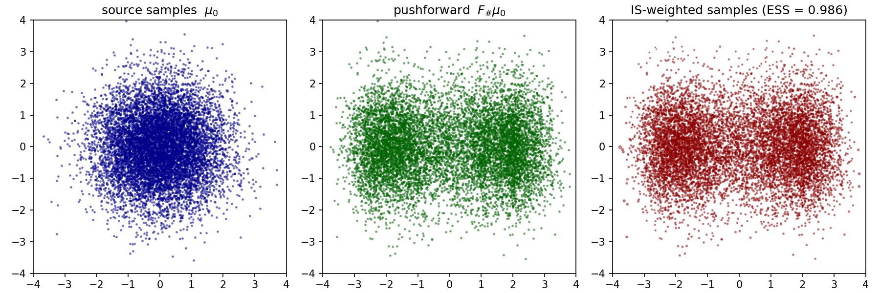
tests/2D_reverse_KL.py (writeup: tests/2D_reverse_KL.md) trains an NSF on a target specified only by an unnormalized energy $U_1(x) = \frac{1}{2}|x|^2 + 2\cos x_1$, then evaluates residual mismatch via importance sampling and $\mathrm{ESS}$.
python -m tests.2D_reverse_KL
2. Data-driven normalizing flow (forward KL)
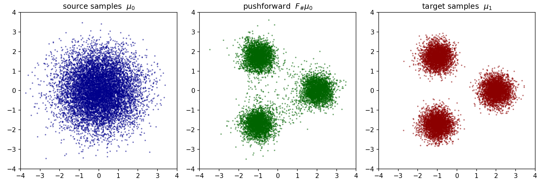
tests/2D_forward_KL.py (writeup: tests/2D_forward_KL.md) trains an NSF on samples from a 3-mode Gaussian mixture — only u1.samples(N) is ever called.
python -m tests.2D_forward_KL
3. Compiled vs. raw forward/inverse map benchmark
tests/compare_compiled_inverse.py (writeup: tests/compare_compiled_inverse.md) benchmarks the compiled ComposedTransform fast paths — F.for_ladj(x) (compiled call_and_ladj) and F.inv_ladj(y) (compiled inv.call_and_ladj), each returning the fused (points, log|det J|) — against the raw flow.t().call_and_ladj(x) / flow.t().inv.call_and_ladj(y) pattern, across an NSF dimension × hidden_features grid. The eager maps are host-overhead-bound at small d, so compiling them is a clean win.
python -m tests.compare_compiled_inverse
Result on an RTX 5070 Ti (committed tests/compare_compiled_inverse.csv). The fwd columns are the forward map flow.t().call_and_ladj(x); the inv columns are the inverse map flow.t().inv.call_and_ladj(y). Within each, the three timing columns are the mean ms per call (over 50 calls) in three modes — raw (no compile, fresh flow.t() each call), def (compiled F.for_ladj/F.inv_ladj with mode='default'), and red (compiled with mode='reduce-overhead', CUDA Graphs) — and the two ↑ columns are the resulting speedups over raw: ↑def = raw / def, ↑red = raw / red. So a row reads: forward map costs fwd raw ms uncompiled and fwd def/fwd red ms compiled, a fwd ↑def/fwd ↑red× speedup; likewise for the inverse map.
| $d$ | hidden_features | fwd raw | fwd def | fwd red | fwd ↑def | fwd ↑red | inv raw | inv def | inv red | inv ↑def | inv ↑red |
|---|---|---|---|---|---|---|---|---|---|---|---|
| 2 | (64, 64) | 1.573 | 0.328 | 0.235 | 4.80 | 6.69 | 4.291 | 0.685 | 0.582 | 6.26 | 7.37 |
| 2 | (128, 128) | 1.602 | 0.309 | 0.308 | 5.18 | 5.20 | 4.260 | 0.780 | 0.792 | 5.46 | 5.38 |
| 2 | (256, 256) | 1.579 | 0.419 | 0.415 | 3.77 | 3.80 | 4.282 | 1.184 | 1.131 | 3.62 | 3.79 |
| 4 | (64, 64) | 1.625 | 0.342 | 0.247 | 4.75 | 6.59 | 7.117 | 1.130 | 1.100 | 6.30 | 6.47 |
| 4 | (128, 128) | 1.611 | 0.331 | 0.329 | 4.87 | 4.89 | 7.059 | 1.457 | 1.439 | 4.84 | 4.90 |
| 4 | (256, 256) | 1.610 | 0.509 | 0.504 | 3.16 | 3.19 | 7.270 | 2.420 | 2.347 | 3.00 | 3.10 |
| 8 | (64, 64) | 3.845 | 0.333 | 0.331 | 11.54 | 11.63 | 32.991 | 2.695 | 2.605 | 12.24 | 12.67 |
| 8 | (128, 128) | 3.975 | 0.484 | 0.435 | 8.22 | 9.14 | 34.049 | 3.715 | 3.569 | 9.17 | 9.54 |
| 8 | (256, 256) | 4.163 | 0.598 | 0.599 | 6.97 | 6.95 | 35.522 | 5.132 | 5.113 | 6.92 | 6.95 |
| 16 | (64, 64) | 6.523 | 0.428 | 0.427 | 15.25 | 15.29 | 107.037 | 6.884 | 6.679 | 15.55 | 16.03 |
| 16 | (128, 128) | 6.561 | 0.513 | 0.512 | 12.79 | 12.81 | 108.207 | 8.285 | 8.035 | 13.06 | 13.47 |
| 16 | (256, 256) | 6.803 | 0.756 | 0.759 | 9.00 | 8.96 | 111.941 | 12.130 | 11.859 | 9.23 | 9.44 |
| 32 | (64, 64) | 11.847 | 0.600 | 0.607 | 19.73 | 19.53 | 384.586 | 19.143 | 18.701 | 20.09 | 20.57 |
| 32 | (128, 128) | 12.053 | 0.771 | 0.772 | 15.62 | 15.61 | 390.656 | 24.547 | 24.225 | 15.91 | 16.13 |
| 32 | (256, 256) | 12.404 | 1.116 | 1.113 | 11.11 | 11.15 | 402.105 | 35.689 | 35.321 | 11.27 | 11.38 |
The speedup grows with d: the forward sees ~3–20× and the inverse spline bisection ~3–21×, largest at $d = 32$ where the raw inverse (~385–402 ms — sequential per-coordinate bisection) collapses to ~19–35 ms. The two compile modes are within noise here (no backward / optimizer, so there is little extra launch overhead for CUDA Graphs to remove). See the writeup for methodology and the re-enable rules.
4. Compiled vs. raw loss benchmark
tests/compare_compiled_loss.py (writeup: tests/compare_compiled_loss.md) sweeps NSF across a dimension × hidden_features grid and times the full training step (forward + backward() + Adam.step()) in three modes: raw reverse_KL(x, target, flow.t()), loss_compile(...) with mode='default', and with mode='reduce-overhead' (CUDA Graphs). The captured-once trick — pass F = flow.t() as a closure constant so Dynamo sees a stable object identity across iterations — turns what looks like a Python-overhead-bound workload at small dimension into a fused CUDA-graph replay.
python -m tests.compare_compiled_loss
Result on an RTX 5070 Ti (committed tests/compare_compiled_loss.csv), mean ms per training step over 100 timed steps:
| dimension | hidden_features | raw ms | default ms | reduce ms | speedup default | speedup reduce |
|---|---|---|---|---|---|---|
| 2 | (64, 64) | 6.03 | 1.41 | 0.50 | 4.30 | 12.18 |
| 2 | (128, 128) | 5.90 | 1.44 | 0.51 | 4.09 | 11.66 |
| 2 | (256, 256) | 6.31 | 1.61 | 0.65 | 3.93 | 9.72 |
| 4 | (64, 64) | 6.28 | 1.52 | 0.56 | 4.12 | 11.24 |
| 4 | (128, 128) | 5.68 | 1.44 | 0.52 | 3.95 | 10.92 |
| 4 | (256, 256) | 5.63 | 1.42 | 0.73 | 3.96 | 7.67 |
| 8 | (64, 64) | 5.38 | 1.46 | 0.56 | 3.69 | 9.68 |
| 8 | (128, 128) | 5.91 | 1.44 | 0.63 | 4.10 | 9.45 |
| 8 | (256, 256) | 6.16 | 1.42 | 0.91 | 4.33 | 6.73 |
| 16 | (64, 64) | 7.56 | 1.49 | 0.68 | 5.08 | 11.12 |
| 16 | (128, 128) | 7.84 | 1.33 | 0.80 | 5.90 | 9.80 |
| 16 | (256, 256) | 7.50 | 1.34 | 1.09 | 5.60 | 6.86 |
| 32 | (64, 64) | 12.16 | 1.31 | 1.12 | 9.26 | 10.91 |
| 32 | (128, 128) | 12.59 | 1.42 | 1.35 | 8.89 | 9.31 |
| 32 | (256, 256) | 12.76 | 1.67 | 1.65 | 7.64 | 7.71 |
The raw baseline starts rising at $d \ge 16$ — by $d = 32$ it has roughly doubled to ~12–13 ms regardless of hidden_features, which is where GPU compute begins to dominate over Python launch overhead. reduce-overhead consistently delivers 6.5–12× per-step speedup; default mode (no CUDA Graphs) delivers ~4–9×. The speedup persists at the largest cell ($d = 32$, hidden_features = (256, 256)) at ~7.5×, well past the point where the bottleneck shifts from Python to compute. See the writeup for the methodology (warmup, sanity check, cache-size limits) and three observations on how the gap scales.
5. Periodic target with rejuvenation
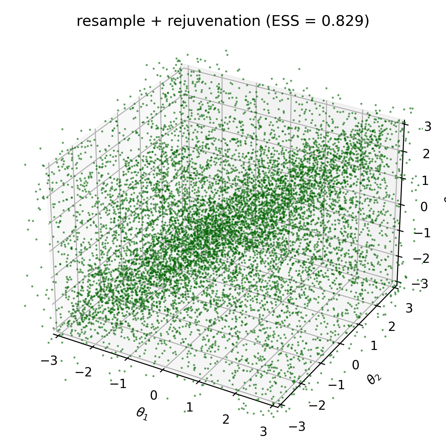
tests/3D_periodic.py (writeup: tests/3D_periodic.md) trains an NCSF on a von-Mises ridge mixture on the 3-torus $[-\pi, \pi]^3$, then runs the full pipeline: importance sampling → resample → enable_grad → Langevin rejuvenation.
python -m tests.3D_periodic
6. Annealed Boltzmann generator (4D, two repelling charges)
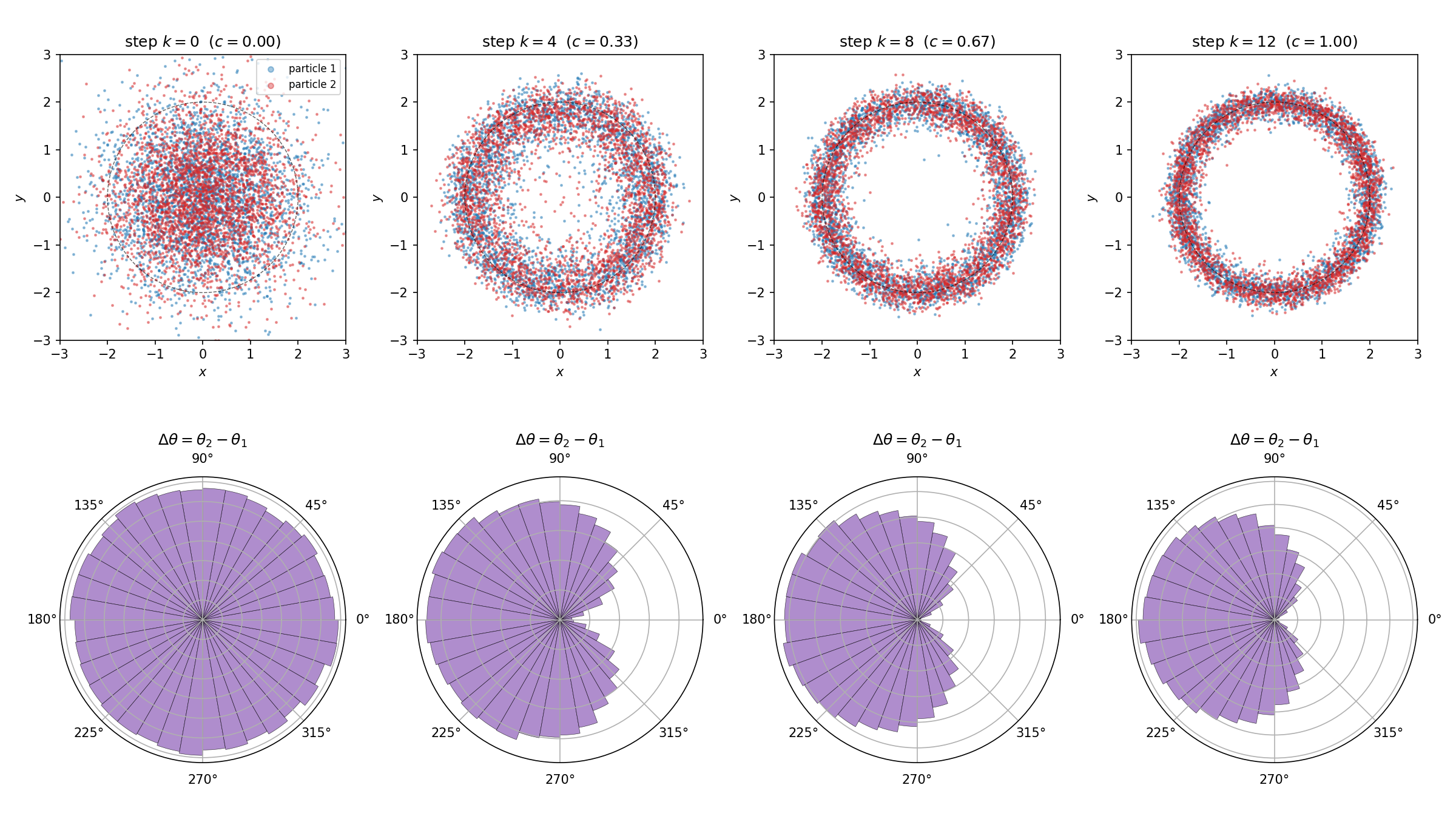
tests/4D_Boltzmann_generator.py (writeup: tests/4D_Boltzmann_generator.md) trains an NSF on the 4D target of two charges in $\mathbb R^2$ confined to a soft annulus and repelling via a regularized 3D Coulomb. A direct flow proposal would have $\mathrm{ESS} \approx 0$, so we anneal: chain .enable_grad() on each constituent potential ($u_{\mathrm{source}}$ and $u_{\mathrm{target}}$) at the very top of the script, build two linear_combination bridge potentials once (the IS denominator $U_{k-1}$ and the training / IS-numerator / MALA target $U_k$ — both auto-inherit the compiled gradient fast path through their __init__-linked closures), and retune coefficients per rung via plain set_coeffs([c, 1-c]). The children's compiled .grad is paid for exactly once at construction time and reused unchanged across all $M{=}12$ rungs. A single hoisted loss_compile(reverse_KL, u_curr, F) handles the per-rung reverse-KL training without per-rung re-instantiation. Each rung runs resample → reverse KL train → IS → resample → MALA rejuvenation, with the same flow warm-started across rungs. ESS climbs from $0.68$ at $k=1$ straight to a $0.96$–$0.97$ plateau by $k=2$ and stays there for the remaining ten rungs. The figure shows the marginal annulus forming (top row) and the joint relative-angle distribution $\Delta\theta = \theta_2 - \theta_1$ on $S^1$ shifting from uniform at $k=0$ to peaked at $\pm\pi$ at $k=12$ — the antipodal Coulomb minimum.
python -m tests.4D_Boltzmann_generator
7. Continuous normalizing flow on two moons (CNF / FFJORD)
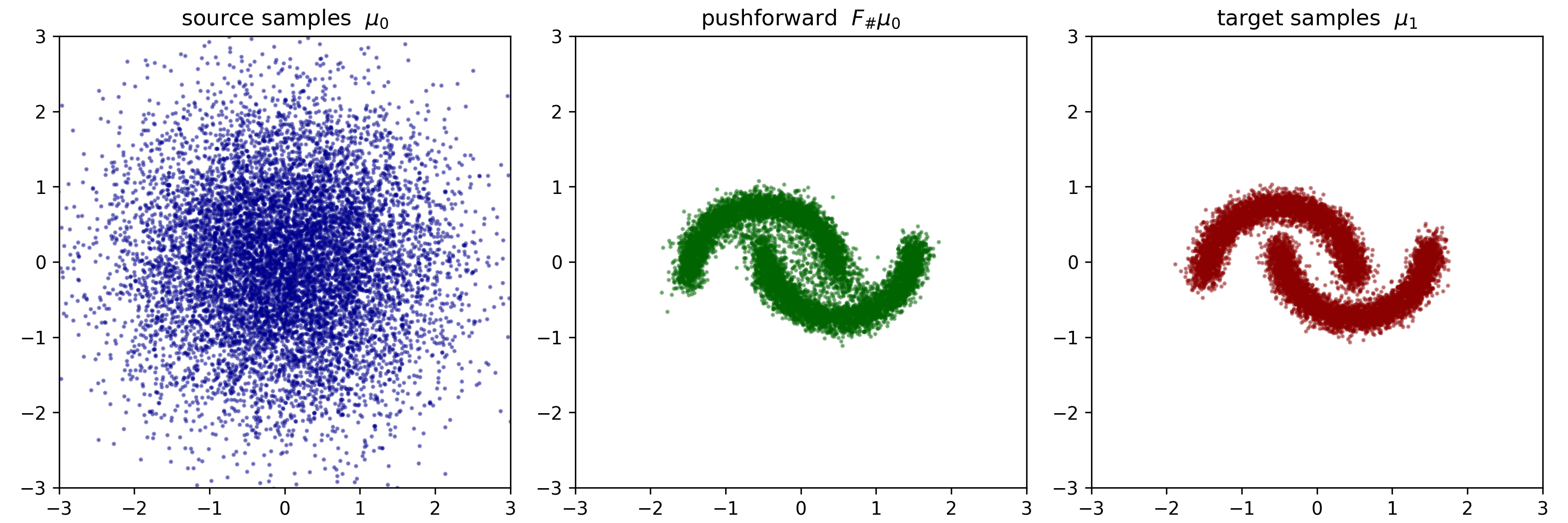
tests/2D_two_moon_CNF.py (writeup: tests/2D_two_moon_CNF.md) trains a CNF (FFJORD-style continuous normalizing flow) by forward KL on samples from the classic two-moons distribution — a target whose interlocking-arc topology cannot be separated along any axis. The point of this test is to (i) exercise the CNF class on a target where its smooth, non-axis-aligned deformation actually pays off, and (ii) make the CNF/NSF trade-off concrete: closed-form O(d) splines vs. an adaptive ODE flow that buys topological flexibility at the cost of 50–500× slower importance sampling. The writeup includes a side-by-side comparison of the two flow classes across the operations a typical energy-based pipeline performs.
python -m tests.2D_two_moon_CNF
8. RealNVP latent-space interpolation
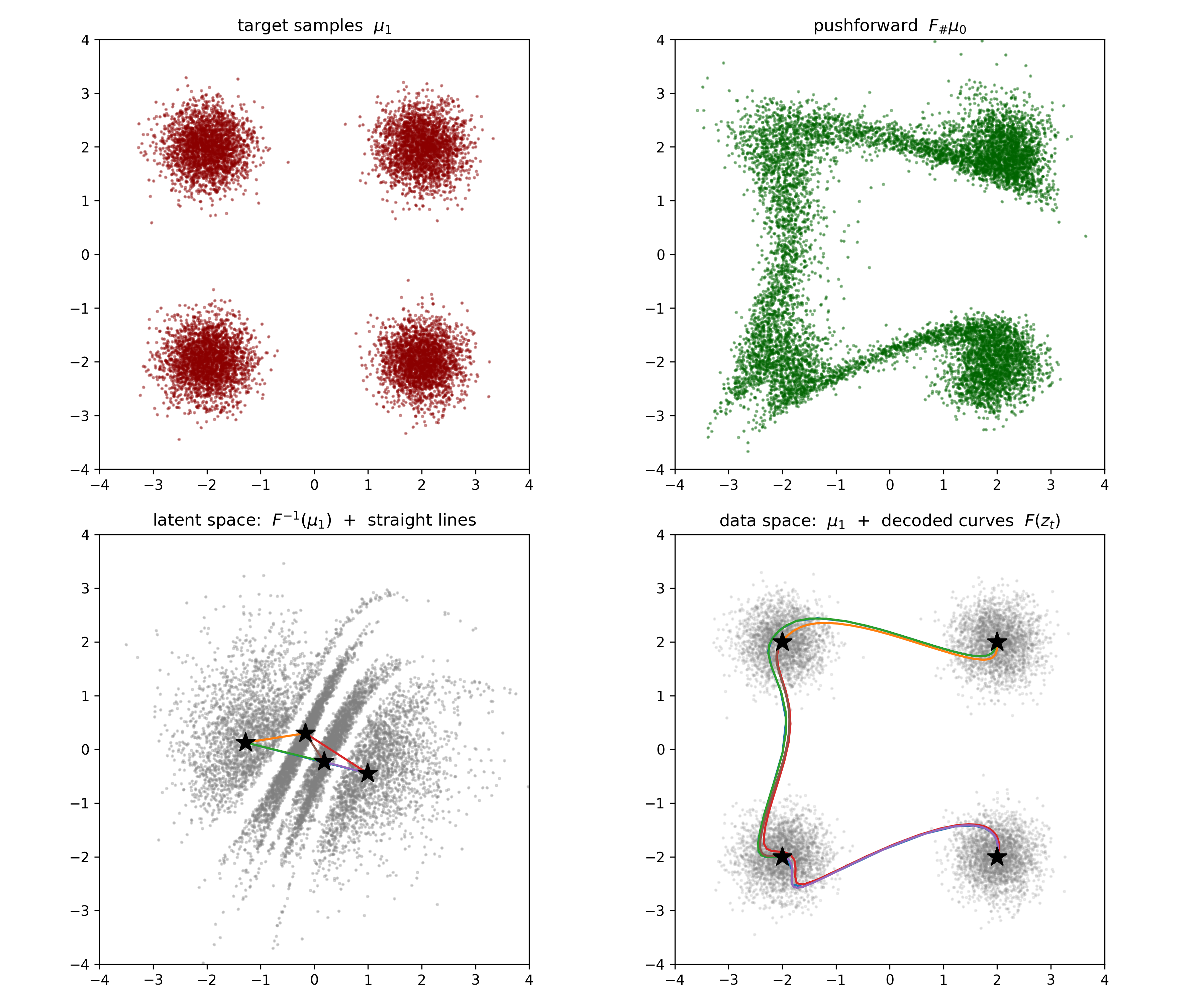
tests/2D_RealNVP_latent_interpolation.py (writeup: tests/2D_RealNVP_latent_interpolation.md) trains a RealNVP by forward KL on a 4-corner Gaussian mixture, then exercises the bijection in the inverse direction: pull each mode center back to the latent space via $z = F^{-1}(x)$, draw straight lines between latent anchors, and decode them with $F$. The decoded curves bend through the data manifold rather than cutting straight across the gaps — the canonical RealNVP morphing demo from Dinh et al. (2016), reduced to 2D so the latent and data spaces are both visible. This is the only test in the folder that puts $F^{-1}$ in the foreground, and the script runs end-to-end only because RealNVP's inverse and log-determinant are closed-form and $O(d)$ — repeating it with NSF (bisection inverse) or CNF (adaptive ODE) would be visibly slower.
python -m tests.2D_RealNVP_latent_interpolation
9. CNF vs. OTFlow on a multi-well target across dimension
tests/multi_well_compare.py (writeup: tests/multi_well_compare.md) pits CNF against OTFlow on the same 8-mode target — the first 3 coordinates are symmetric double wells ($2^3 = 8$ modes), the rest standard Gaussian — trained by the same plain reverse_KL (OTFlow's OT regularizers switched off), warm-started at the identity, with the same fixed-step RK4 budget. It isolates the one variable that differs, the velocity-field architecture, and reports the importance-sampling $\mathrm{ESS}$ of the trained proposal as the dimension grows. The wells are kept shallow so mode-seeking reverse KL must cover all 8 modes rather than collapse onto a subset.
ESS (RTX 5070 Ti, fp32; reproduced from multi_well_compare.csv):
| flow | $d=4$ | $d=8$ | $d=12$ | $d=16$ | $d=20$ | $d=24$ |
|---|---|---|---|---|---|---|
CNF |
0.8939 | 0.8937 | 0.8729 | 0.8667 | 0.6762 | 0.4425 |
OTFlow |
0.9823 | 0.9774 | 0.9735 | 0.9505 | 0.9575 | 0.9621 |
OTFlow holds $\mathrm{ESS} \approx 0.95$–$0.98$ flat across the sweep, while CNF starts comparable but collapses as $d$ grows ($0.89 \to 0.44$ by $d=24$) — the high-dimensional payoff of the closed-form-trace gradient-field parameterisation. At $d \leq 24$ this is a quality win, not a speed one: both flows are launch-overhead-bound, so per-step cost just tracks the chosen nt / hidden / step count.
python -m tests.multi_well_compare
FAQ
Q: What platforms does zflows run on?
Linux + NVIDIA GPU is required. The package has been tested on Ubuntu, Arch, and WSL (Windows Subsystem for Linux); other major Linux distributions should work as well as long as a CUDA-enabled PyTorch build is available.
Native Windows is not supported: torch.compile — the backbone of Potential.enable_grad and loss_compile / loss_compile_beta — does not run on Windows, see pytorch/pytorch#167062. On Windows machines, either use WSL (recommended) or avoid every compile entry point: skip enable_grad (fall back to standard autograd for Potential gradients) and skip loss_compile / loss_compile_beta (call reverse_KL(x, target, flow.t()) raw in your training loop instead). The un-compiled paths are slower but functionally equivalent — every numerical result the test suite produces is identical with or without compile.
macOS is untested. The pure-Python flow / loss code should import and run on the CPU, but the compiled fast paths target CUDA and have not been exercised on Apple Silicon.
Q: How do I check whether torch.compile will actually work in my environment before I burn an hour on training?
Run zflows.utils.check_compile_available() interactively (or in a one-off standalone script — don't put it in your main training code, since each call really invokes torch.compile and consumes a Dynamo cache slot):
>>> import zflows
>>> zflows.utils.check_compile_available()
[OK ]   OS = Linux
[OK ]   nvcc = /opt/cuda/bin/nvcc
[OK ]   sanity test passed (device=cuda, mode=reduce-overhead)
True
It runs three checks: (1) OS is Linux — non-Linux emits a warning but doesn't fail; (2) nvcc is reachable — shutil.which("nvcc") first, then the Ubuntu default install locations /usr/local/cuda/bin/nvcc and /usr/local/cuda-*/bin/nvcc as fallbacks; warns if none match; (3) the authoritative step: actually torch.compile's a small probe function under the same mode='reduce-overhead' zflows uses internally, and returns True iff that succeeds.
The first two checks are warnings only; the bool return value reflects only the sanity test. Failure on (2) is the most common cause of the "C compiler not found" / "nvcc not found" errors that surface on the first call to Potential.enable_grad / loss_compile / loss_compile_beta: torch.compile invokes Triton / TorchInductor, which JIT-compiles a small CUDA helper at first call, and that step needs the NVIDIA C/C++ compiler nvcc from the CUDA Toolkit (not just the CUDA runtime that ships with the PyTorch wheel). Install the toolkit through your distro's package manager or from NVIDIA's downloads page; if the toolkit lives at the Ubuntu default /usr/local/cuda/bin/nvcc or /usr/local/cuda-X.Y/bin/nvcc the fallback picks it up automatically, otherwise add it to $PATH and re-run check_compile_available().
Q: Why is torch.compile so slow — the first call hangs for ages, especially the flow inverse?
That wait is compile time, paid once, not per-step runtime. The first call to any compiled path (Potential.enable_grad / enable_eval, ComposedTransform.enable_for_ladj / enable_inv_ladj, loss_compile) triggers Dynamo tracing → TorchInductor lowering → Triton kernel codegen (+ autotuning under mode='reduce-overhead'). For a training run with thousands of steps this amortizes within the first epoch; for a 10-step toy script it is net-negative, so just skip the enable_* calls there.
The pathological case is the NSF / NCSF inverse (enable_inv_ladj): the spline bisection unrolls into a very large graph, and the compile time grows sharply with dimension and conditioner width — at something like d = 256, hidden_features = (256, 256) it can be extremely slow to compile, and there is no effective way around it (the forward map and the closed-form/ODE inverses of RealNVP / CNF / OTFlow compile fine). If you hit this, the fix is simply to not compile that map: drop the enable_inv_ladj / enable_for_ladj call and use the plain flow.t().inv.call_and_ladj(y) / flow.t().call_and_ladj(x) — the result is identical, only the one-time compile cost disappears.
Things that help the rest of the time: prefer mode='default' (no CUDA-Graph capture or kernel autotuning — much faster to compile, ~10–30% slower at steady state) when compile time matters more than peak throughput; keep a stable batch shape so you don't pay repeated retraces (set_cache_size_limit(64) if you legitimately sweep many shapes/closures); and call suppress_warnings() before the first compile so the long wait isn't also buried in Triton/Inductor log noise.
Q: My runs are buried under warnings — _POSIX_C_SOURCE redefined, Triton autotune banners, TF32 hints, Dynamo recompile logs. How do I silence them all?
Put one line at the top of your script, before any torch.compile invocation:
from zflows.utils import suppress_warnings
suppress_warnings()
This is the single entry point that turns off all four orthogonal layers of noise the PyTorch / Triton / Inductor stack emits during a typical compile-heavy training run:
- Python
UserWarnings — e.g. inductor's TF32 hint,torch.distributionsdeprecation notes — silenced viawarnings.filterwarnings("ignore"). - Dynamo log channels —
recompilesandgraph_breaks— silenced viatorch._logging.set_logs(recompiles=False, graph_breaks=False). - Triton autotune stderr — the per-kernel
AUTOTUNE addmm(...)banners that Triton's C-side autotuner writes directly to stderr (Python'swarningsfilter can't catch these) — silenced viaTRITON_PRINT_AUTOTUNING=0. - Inductor compile-worker interleaving — the
_POSIX_C_SOURCE redefinedwarnings emitted by GCC for every kernel autotuned, plus other gcc/nvcc diagnostics — serialised to one worker viaTORCHINDUCTOR_COMPILE_THREADS=1, so any remaining diagnostic comes out cleanly instead of as interleaved gibberish across N workers.
These layers are orthogonal: Python warning filters don't catch stderr writes from Triton's C side, and torch._logging doesn't catch GCC diagnostics. suppress_warnings() covers all four; the env-var-based pieces (#3 and #4) only take effect for future compiles, so call this before any torch.compile / Potential.enable_grad / loss_compile / loss_compile_beta invocation.
The function is idempotent and safe to call multiple times. Real compile failures still raise — only routine noise is muted. You can see it in action at the top of every test script in tests/ (e.g. tests/3D_periodic.py, tests/_verify_utils.py).
Q: My custom loss function doesn't match the (x, potential, transform) signature of reverse_KL / forward_KL — how do I compile it?
loss_compile(loss_fn, *captured, mode='default') is variadic — it captures every positional argument after loss_fn as a closure constant, so any callable of the form loss_fn(x, *captured) -> scalar works:
from zflows.loss import loss_compile

def my_loss(x, target_potential, transform, scale):
    y, ladj = transform.call_and_ladj(x)
    return (scale * target_potential(y) - ladj).mean()

F = flow.t()
loss_fn = loss_compile(my_loss, u_target, F, 0.5)   # captured = (u_target, F, 0.5)

for x_batch in batches:
    loss = loss_fn(x_batch)
    optimizer.zero_grad(); loss.backward(); optimizer.step()
The pattern that doesn't work is torch.compile(my_loss) and then passing the flow / potentials as runtime arguments — each call would build a fresh flow.t(), Dynamo would re-guard on its object identity, and the cache would either thrash or hit BACKEND_MATCH failures. loss_compile sidesteps both by stuffing the Python-heavy arguments into the closure. If you mix multiple distinct loss-function shapes in the same script, raise torch._dynamo.config.cache_size_limit (or use the helper zflows.utils.set_cache_size_limit(N)) so Dynamo doesn't evict your specializations.
If your loss takes keyword-only arguments or needs more elaborate dispatch, write a thin wrapper that closes over them and pass the wrapper into loss_compile. This is the kind of small mechanical refactor that AI coding assistants (e.g. Claude Code, which built this project) handle well.
Q: Does zflows support conditional normalizing flows?
No. zflows is designed for Boltzmann-generator / energy-based sampling, where you train one flow against one unconditional target distribution. The context / conditional-on-c plumbing that general-purpose flow libraries carry is dead weight in this setting, so it was dropped on purpose when porting the core machinery from zuko — see the package docstring in zflows/__init__.py.
If you need conditional flows, use zuko directly. Its Flow / Transform / masked-MLP machinery is the same shape as what zflows.core vendors — what we removed was just the context argument threaded through every layer — so the API will feel familiar, and zuko has been hardened for the conditional-density-estimation / SBI use cases that motivated it.
Q: I'm using JAX rather than PyTorch — how can I implement normalizing flows?
zflows is PyTorch-only and has no plans to port. For JAX you have two solid options:
- Distrax (recommended) — DeepMind's JAX/TFP-style probability and bijector library. Officially maintained inside Google's open-source stack, broad bijector coverage (RQS, affine, masked autoregressive, etc.), and the API mirrors
tensorflow_probability.substrates.jaxso it composes cleanly with the rest of the JAX/Flax/Haiku ecosystem. - FlowJAX — flow-focused library by Daniel Ward, smaller surface area but ergonomic for the common "fit a flow to samples or a target density" workflow.
Neither is a drop-in replacement for the energy-based sampling / Boltzmann-generator pipeline zflows is built around — both target the SBI / density-estimation use cases — so expect to assemble the propose → reweight → resample → rejuvenate loop yourself out of their primitives.
On raw speed: with torch.compile in the training loop (via loss_compile / loss_compile_beta / Potential.enable_grad), the per-step gap between JAX and PyTorch is typically minor. What PyTorch still gives you for free is a natural OOP layout centered on nn.Module — Flow, Potential, and their subclasses all inherit from it, so .to(device), .parameters(), .state_dict(), and optimizer.step() work without extra plumbing. JAX has no equivalent default and routes parameters explicitly. Random number generation is similar: PyTorch's global torch.manual_seed(...) is sufficient for the Langevin / MALA / HMC routines in zflows.utils, while JAX requires you to thread a PRNGKey through every sampler call.
Q: How can I apply zflows on real molecules rather than the toy examples?
The maintainer is working to combine zflows with torchmd and openmm so that a real Amber-style full-atom potential plugs in as a zflows.Potential subclass.
Acknowledgements
zflows is strongly inspired by zuko; the flow, transform, and masked-MLP machinery vendored into zflows.core is a stripped-down port of zuko's. Credit for the underlying design — and for the clean, composable Transform API the public flows build on — belongs to the zuko authors.
Project details
Verified details
These details have been verified by PyPIProject links
GitHub Statistics
Maintainers


Download files
Download the file for your platform. If you're not sure which to choose, learn more about installing packages.
Source Distribution
Built Distribution
Filter files by name, interpreter, ABI, and platform.
If you're not sure about the file name format, learn more about wheel file names.
Copy a direct link to the current filters
File details
Details for the file zflows-0.6.2.tar.gz.
File metadata
- Download URL: zflows-0.6.2.tar.gz
- Upload date:
- Size: 102.8 kB
- Tags: Source
- Uploaded using Trusted Publishing? Yes
- Uploaded via: twine/6.1.0 CPython/3.13.12
File hashes
| Algorithm | Hash digest | |
|---|---|---|
| SHA256 |
3a28764749e348e86e66edb88626a33a77fcc231f7bcd24a629d36004ecca03d
|
|
| MD5 |
de4fd6b6d2c8a4173b09cfb825a94887
|
|
| BLAKE2b-256 |
aa57934b68bb68ea751697b577b60e3ba675d99fa4ee274891e4fe8ee2220baf
|
Provenance
The following attestation bundles were made for zflows-0.6.2.tar.gz:
Publisher:
publish-to-pypi.yml on xuda-ye-math/zflows
-
Statement:
-
Statement type:
https://in-toto.io/Statement/v1 -
Predicate type:
https://docs.pypi.org/attestations/publish/v1 -
Subject name:
zflows-0.6.2.tar.gz -
Subject digest:
3a28764749e348e86e66edb88626a33a77fcc231f7bcd24a629d36004ecca03d - Sigstore transparency entry: 1727886112
- Sigstore integration time:
-
Permalink:
xuda-ye-math/zflows@573f7c5cd4a15e7316cdba60799c78322cddbfef -
Branch / Tag:
refs/tags/v0.6.2 - Owner: https://github.com/xuda-ye-math
-
Access:
public
-
Token Issuer:
https://token.actions.githubusercontent.com -
Runner Environment:
github-hosted -
Publication workflow:
publish-to-pypi.yml@573f7c5cd4a15e7316cdba60799c78322cddbfef -
Trigger Event:
push
-
Statement type:
File details
Details for the file zflows-0.6.2-py3-none-any.whl.
File metadata
- Download URL: zflows-0.6.2-py3-none-any.whl
- Upload date:
- Size: 77.7 kB
- Tags: Python 3
- Uploaded using Trusted Publishing? Yes
- Uploaded via: twine/6.1.0 CPython/3.13.12
File hashes
| Algorithm | Hash digest | |
|---|---|---|
| SHA256 |
512bcb8a761d7000024864a111e3466852bf79068f6111fb6f9f41eb3541a014
|
|
| MD5 |
57ed5eb3b12c9fcabbd1c8449f496a3a
|
|
| BLAKE2b-256 |
d1174a660ff5fc43c8f3a808b280eace3912daae84549c8144d02365f0c7721a
|
Provenance
The following attestation bundles were made for zflows-0.6.2-py3-none-any.whl:
Publisher:
publish-to-pypi.yml on xuda-ye-math/zflows
-
Statement:
-
Statement type:
https://in-toto.io/Statement/v1 -
Predicate type:
https://docs.pypi.org/attestations/publish/v1 -
Subject name:
zflows-0.6.2-py3-none-any.whl -
Subject digest:
512bcb8a761d7000024864a111e3466852bf79068f6111fb6f9f41eb3541a014 - Sigstore transparency entry: 1727886183
- Sigstore integration time:
-
Permalink:
xuda-ye-math/zflows@573f7c5cd4a15e7316cdba60799c78322cddbfef -
Branch / Tag:
refs/tags/v0.6.2 - Owner: https://github.com/xuda-ye-math
-
Access:
public
-
Token Issuer:
https://token.actions.githubusercontent.com -
Runner Environment:
github-hosted -
Publication workflow:
publish-to-pypi.yml@573f7c5cd4a15e7316cdba60799c78322cddbfef -
Trigger Event:
push
-
Statement type:






