




Installation
There are a couple ways in which you can use this library. The first and probably the easiest is by using pip and PyPi:
pip install landscapes
You can also install directly from this git repo:
pip install git+https://github.com/nathanrooy/landscapes
Lastly, you can always clone/download this repo and use as is.
wget https://github.com/nathanrooy/landscapes/archive/master.zip
unzip master.zip
cd landscapes-master
Available functions from: single_objective
| function name | method | dimensions |
|---|---|---|
| Ackley | ackley() |
2 |
| Ackley N.2 | ackley_n2() |
2 |
| Adjiman | adjiman() |
2 |
| AMGM | amgm() |
n |
| Bartels Conn | bartels_conn() |
2 |
| Bird | bird() |
2 |
| Beale | beale() |
2 |
| Bent Cigar | bent_cigar() |
n |
| Bohachevsky N.1 | bohachevsky_n1() |
2 |
| Bohachevsky N.2 | bohachevsky_n2() |
2 |
| Bohachevsky N.3 | bohachevsky_n3() |
2 |
| Booth | booth() |
2 |
| Branin | branin() |
2 |
| Brent | brent() |
2 |
| Brown | brown() |
n |
| Bukin n6 | bukin_n6() |
2 |
| 3-Hump Camel | camel_hump_3() |
2 |
| 6-Hump Camel | camel_hump_6() |
2 |
| Carrom Table | carrom_table() |
2 |
| Chichinadze | chichinadze() |
2 |
| Chung Reynolds | chung_reynolds() |
n |
| Colville | colville() |
4 |
| Cosine Mixture | cosine_mixture() |
n |
| Cross-in-Tray | cross_in_tray() |
2 |
| Csendes | csendes() |
n |
| Cube | cube() |
2 |
| Damavandi | damavandi() |
2 |
| Deckkers-Aarts | deckkers_aarts() |
2 |
| Dixon & Price | dixon_price() |
n |
| Drop Wave | drop_wave() |
2 |
| Easom | easom() |
2 |
| Eggholder | eggholder() |
2 |
| Exponential | exponential() |
n |
| Freudenstein Roth | freudenstein_roth() |
2 |
| Goldstein–Price | goldstein_price() |
2 |
| Griewank | griewank() |
n |
| Himmelblau | himmelblau() |
2 |
| Hölder table | holder_table() |
2 |
| Hosaki | hosaki() |
2 |
| Keane | keane() |
2 |
| Leon | leon() |
2 |
| Lévi function N.13 | levi_n13() |
2 |
| Matyas | matyas() |
2 |
| Michalewicz | michalewicz |
n |
| McCormick | mccormick() |
2 |
| Parsopoulos | parsopoulos() |
2 |
| Pen Holder | pen_holder() |
2 |
| Plateau | plateau() |
n |
| Qing | qing() |
n |
| Quartic | quartic() |
n |
| Rastrigin | rastrigin() |
n |
| Rotated Hyper-Ellipsoid | rotated_hyper_ellipsoid() |
n |
| Rosenbrock | rosenbrock() |
n |
| Salomon | salomon() |
n |
| Schaffer N.2 | schaffer_n2() |
2 |
| Schaffer N.4 | schaffer_n4() |
2 |
| Schwefel | schwefel() |
n |
| Sphere | sphere() |
n |
| Step | step() |
n |
| Styblinski–Tang | styblinski_tang() |
n |
| Sum of Different Powers | sum_of_different_powers() |
n |
| Sum of Squares | sum_of_squares() |
n |
| Trid | trid() |
n |
| Tripod | tripod() |
2 |
| Wolfe | wolfe() |
3 |
| Zakharov | zakharov() |
n |
Usage
As a simple example, let's use the Nelder-Mead method via SciPy to minimize the sphere function. We'll start off by importing the sphere function from Landscapes and the minimize method from SciPy.
>>> from landscapes.single_objective import sphere
>>> from scipy.optimize import minimize
Next, we'll call the minimize method using a starting location of [5,5].
>>> minimize(sphere, x0=[5,5], method='Nelder-Mead')
The output of which should look close to this:
 final_simplex: (array([[-3.33051318e-05, -1.93825710e-05],
       [ 4.24925225e-05,  1.37129516e-05],
       [ 3.09383247e-05, -4.04797876e-05]]), array([1.48491586e-09, 1.99365951e-09, 2.59579314e-09]))
           fun: 1.4849158640215086e-09
       message: 'Optimization terminated successfully.'
          nfev: 80
           nit: 44
        status: 0
       success: True
             x: array([-3.33051318e-05, -1.93825710e-05])
Function Reference - Single Objective
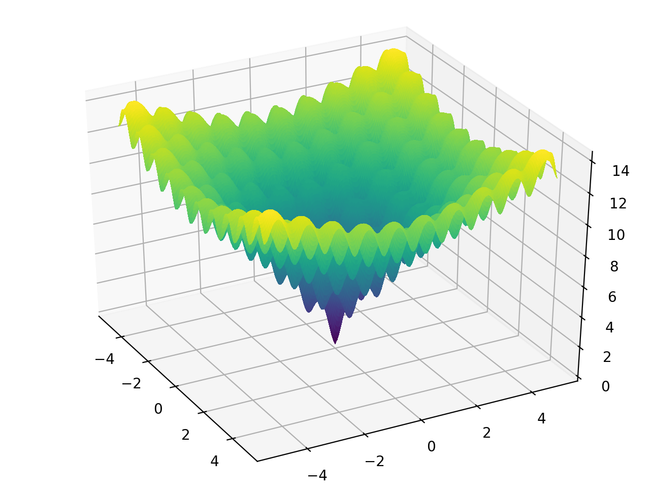
Ackley function
from landscapes.single_objective import ackley
| global minimum | bounds | usage |
|---|---|---|
| f(x=0,y=0)=0 | -5.12 <= x, y <= 5.12 | ackley([x,y]) |
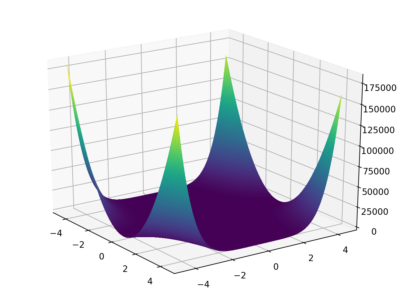
Beale function
from landscapes.single_objective import beale
| global minimum | bounds | usage |
|---|---|---|
| f(x=3, y=0.5) = 0 | -4.5 <= x, y <= 4.5 | beale([x,y]) |
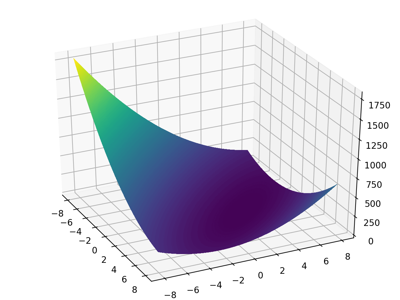
Booth function
from landscapes.single_objective import booth
| global minimum | bounds | usage |
|---|---|---|
| f(x=1, y=3) = 0 | -10 <= x, y <= 10 | booth([x,y]) |
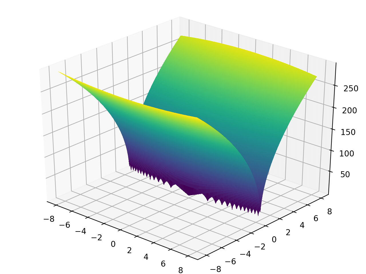
Bukin N.6 function
from landscapes.single_objective import bukin_n6
| global minimum | bounds | usage |
|---|---|---|
| f(x=-10, y=1) = 0 | -15 <= x <= -5 -3 <= y <= 3 |
bukin_n6([x,y]) |
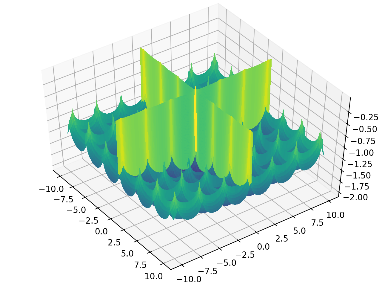
Cross-in-tray function
from landscapes.single_objective import cross_in_tray
| global minimum(s) | bounds | usage |
|---|---|---|
| f(x=1.34941, y=-1.34941) = -2.06261 f(x=1.34941, y=1.34941) = -2.06261 f(x=-1.34941, y=1.34941) = -2.06261 f(x=-1.34941, y=-1.34941) = -2.06261 |
-10 <= x, y <= 10 | cross_in_tray([x,y]) |
Easom function
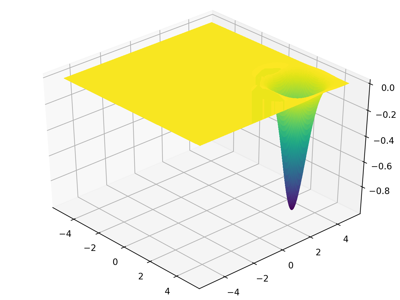
from landscapes.single_objective import easom
| global minimum | bounds | usage |
|---|---|---|
| f(x=pi, y=pi) = -1 | -100 <= x, y <= 100 | easom([x,y]) |
Eggholder function
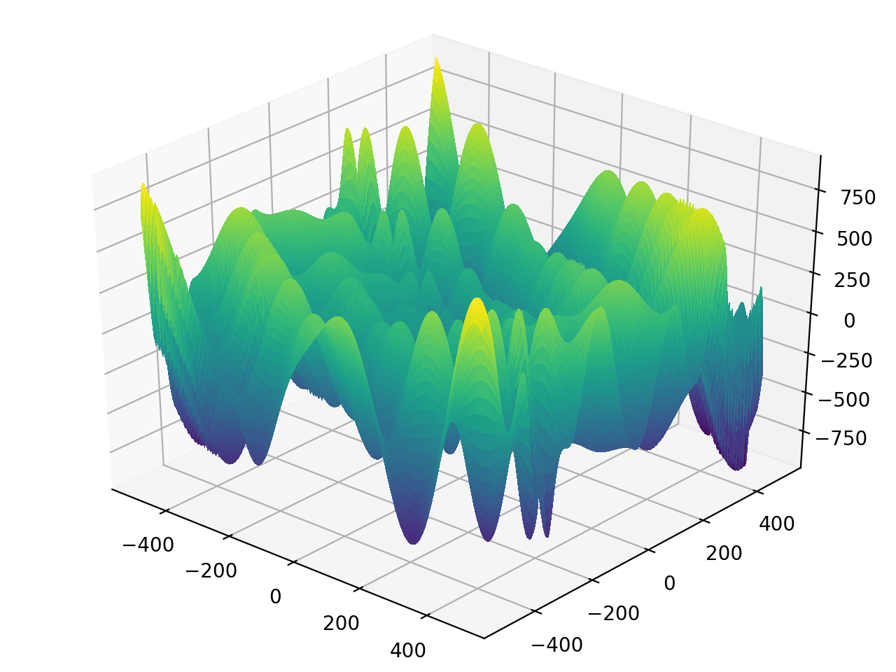
from landscapes.single_objective import eggholder
| global minimum | bounds | usage |
|---|---|---|
| f(x=512, y=404.2319) = -959.6407 | -512 <= x, y <= 512 | eggholder([x,y]) |
Goldstein–Price function
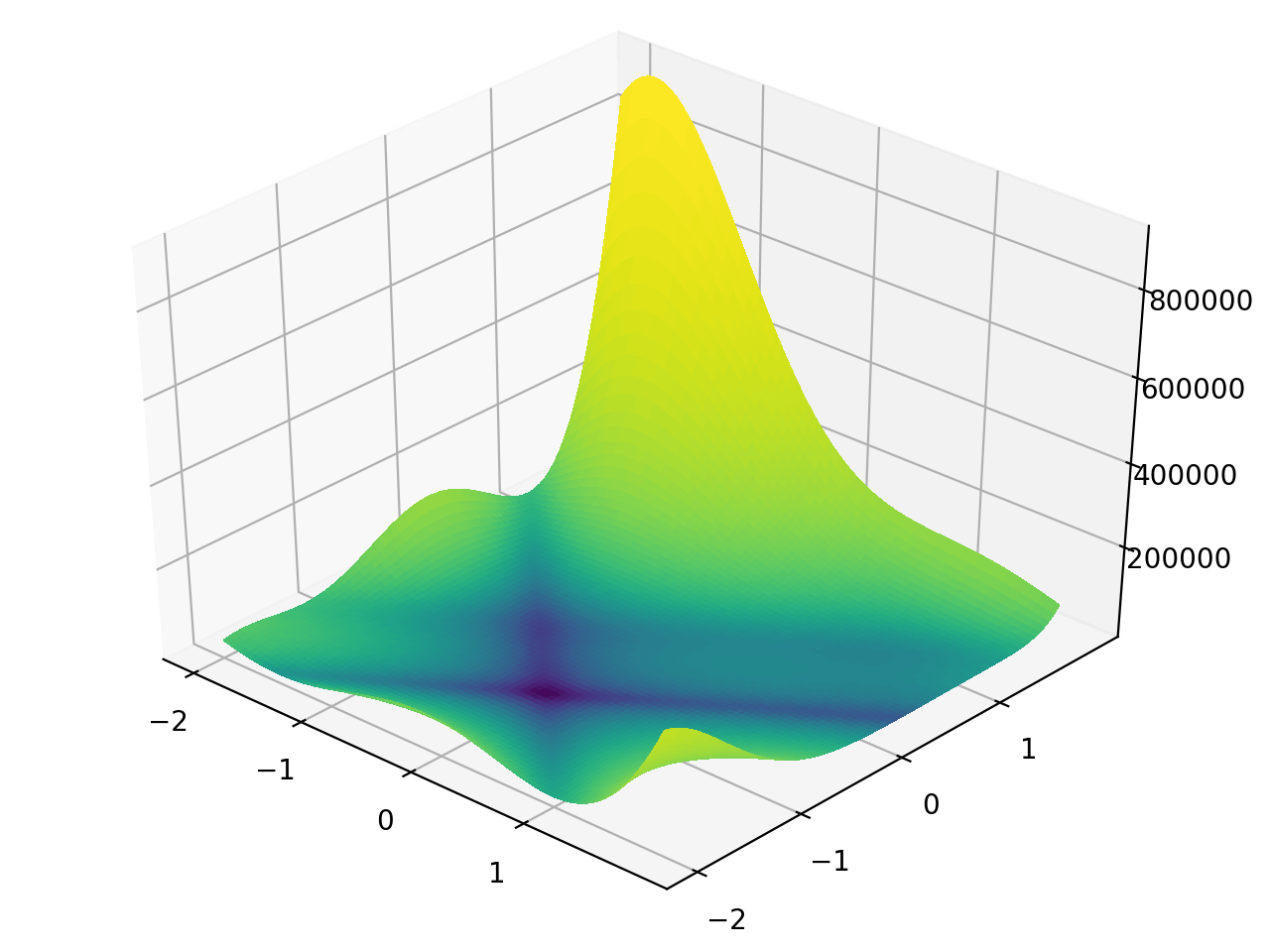
from landscapes.single_objective import goldstein_price
| global minimum | bounds | usage |
|---|---|---|
| f(x=0, y=-1) = 3 | -2 <= x, y <= 2 | goldstein_price([x,y]) |
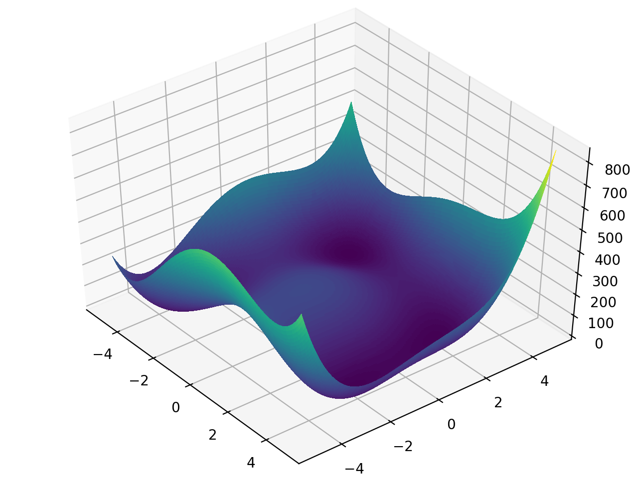
Himmelblau's function
from landscapes.single_objective import himmelblau
| global minimum(s) | bounds | usage |
|---|---|---|
| f(x=3.0, y=2.0) = 0.0 f(x=-2.805118, y=3.131312) = 0.0 f(x=-3.779310, y=-3.283186) = 0.0 f(x=3.584428, y=-1.848126) = 0.0 |
-5 <= x, y <= 5 | himmelblau([x,y]) |
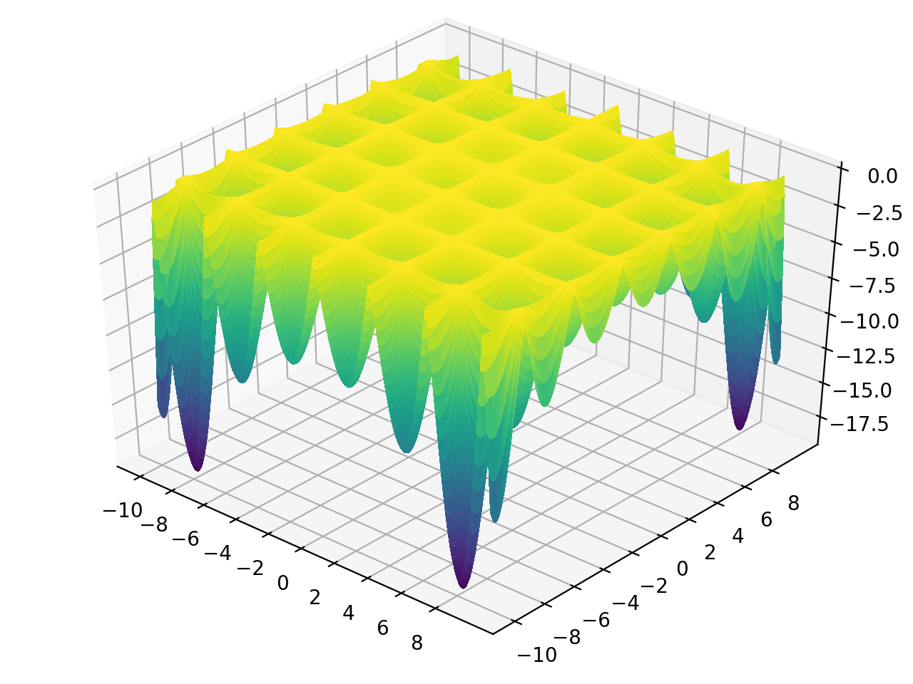
Hölder table function
from landscapes.single_objective import holder_table
| global minimum(s) | bounds | usage |
|---|---|---|
| f(x=8.05502, y=9.66459) = -19.2085 f(x=-8.05502, y=9.66459) = -19.2085 f(x=8.05502, y=-9.66459) = -19.2085 f(x=-8.05502, y=-9.66459) = -19.2085 |
-10 <= x, y <= 10 | holder_table([x,y]) |
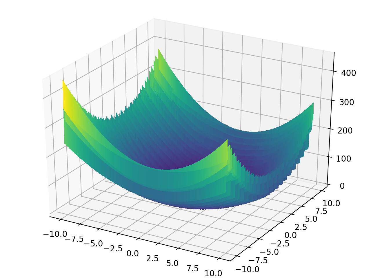
Lévi function N.13
from landscapes.single_objective import levi_n13
| global minimum | bounds | usage |
|---|---|---|
| f(x=1, y=1) = 0 | -10 <= x, y <= 10 | levi_n13([x,y]) |
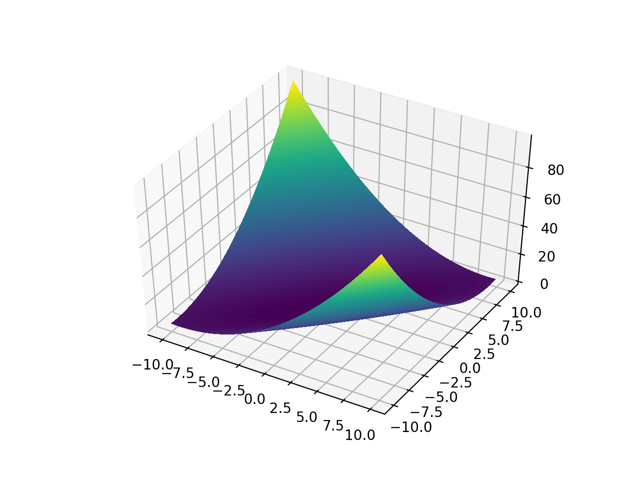
Matyas function
from landscapes.single_objective import matyas
| global minimum | bounds | usage |
|---|---|---|
| f(x=0, y=0) = 0 | -10 <= x, y <= 10 | matyas([x,y]) |
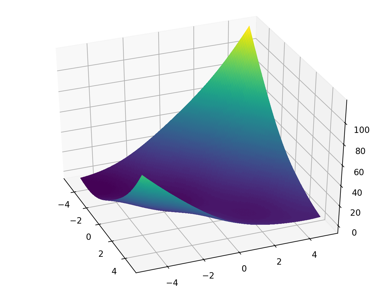
McCormick function
from landscapes.single_objective import mccormick
| global minimum | bounds | usage |
|---|---|---|
| f(x=-0.54719, y=-1.54719) = -1.9133 | -1.5 <= x <= 4 -3 <= y <= 4 |
mccormick([x,y]) |
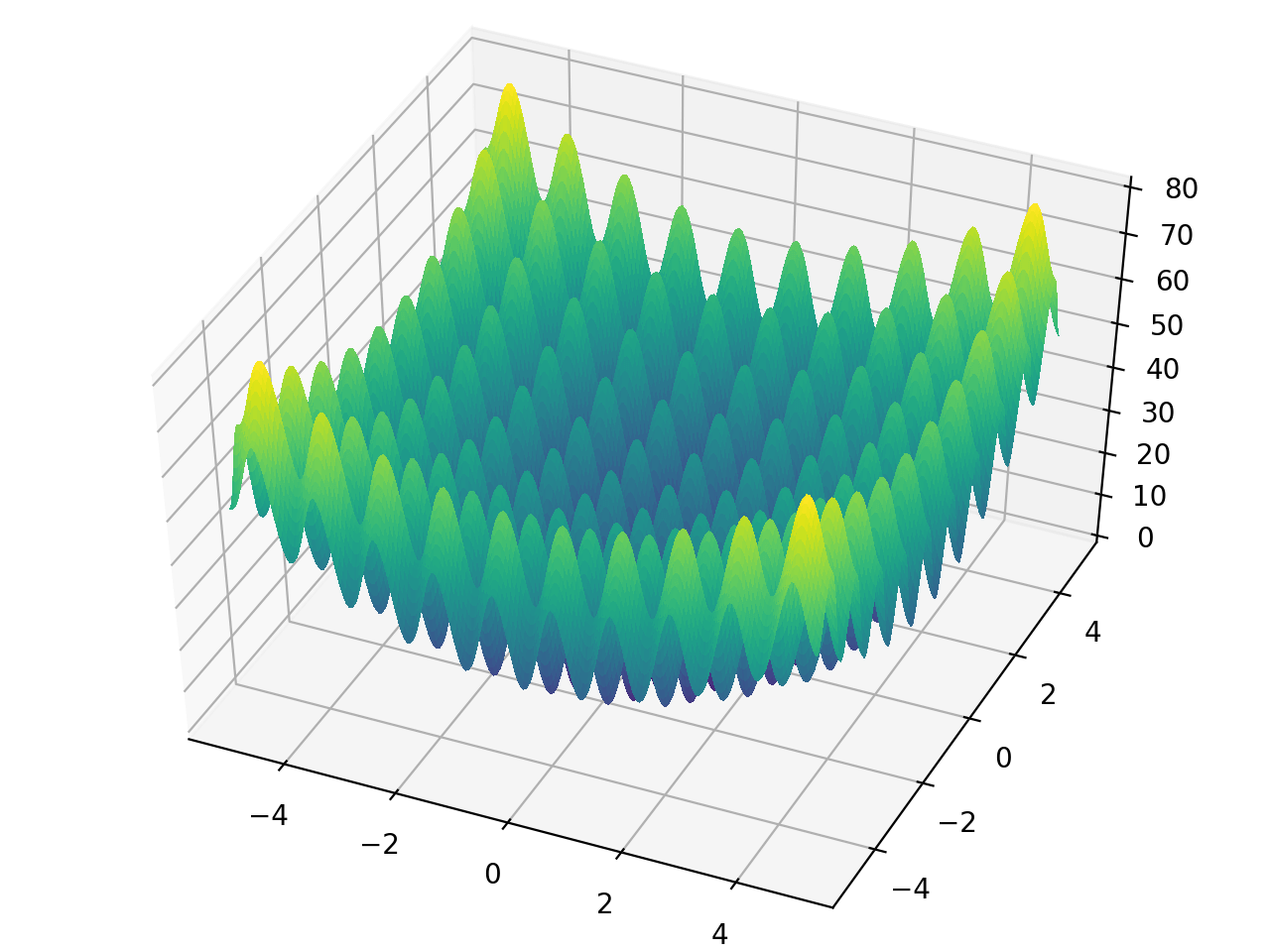
Rastrigin function
from landscapes.single_objective import rastrigin
| global minimum | bounds | usage |
|---|---|---|
| f([0,...,0]) = 0 | -5.12 <= x_i <= 5.12 | rastrigin([x_1,...,x_n]) |
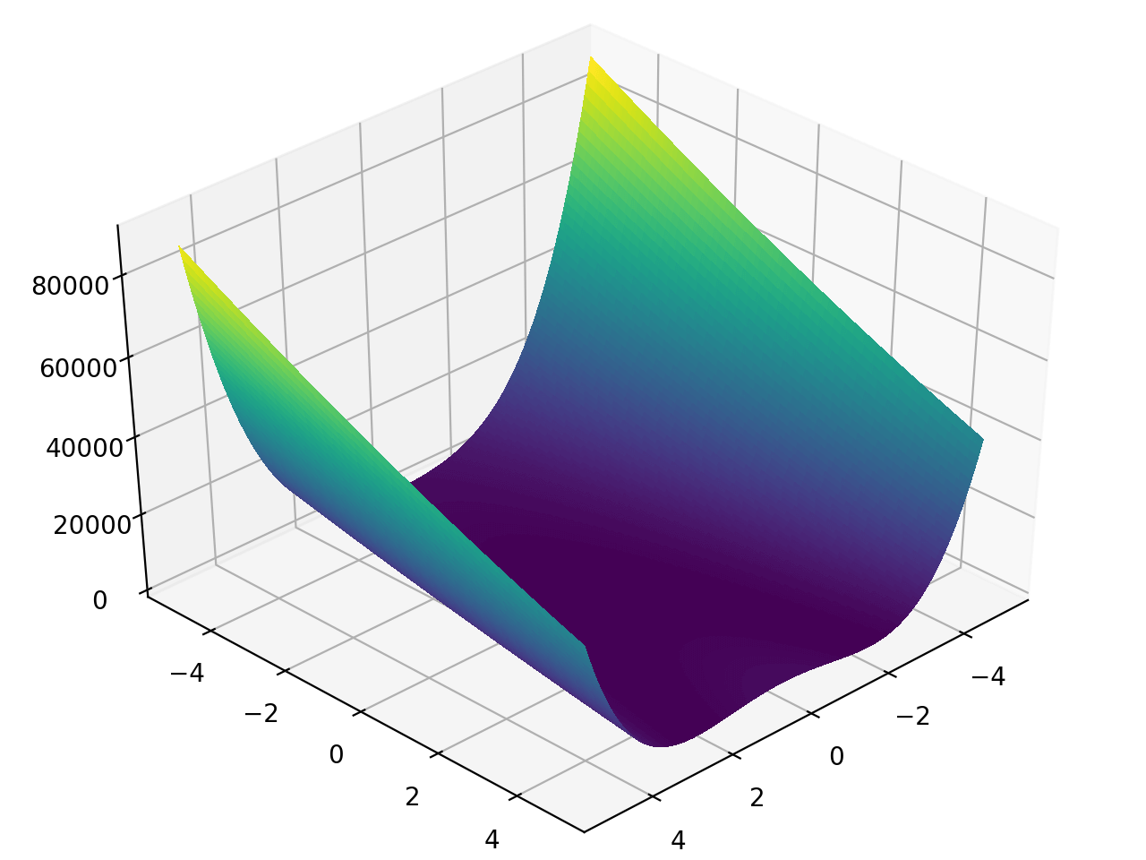
Rosenbrock function
from landscapes.single_objective import rosenbrock
| global minimum | bounds | usage |
|---|---|---|
| f([1,...,1]) = 0 | -inf <= x_i <= inf | rosenbrock([x_1,...,x_n]) |
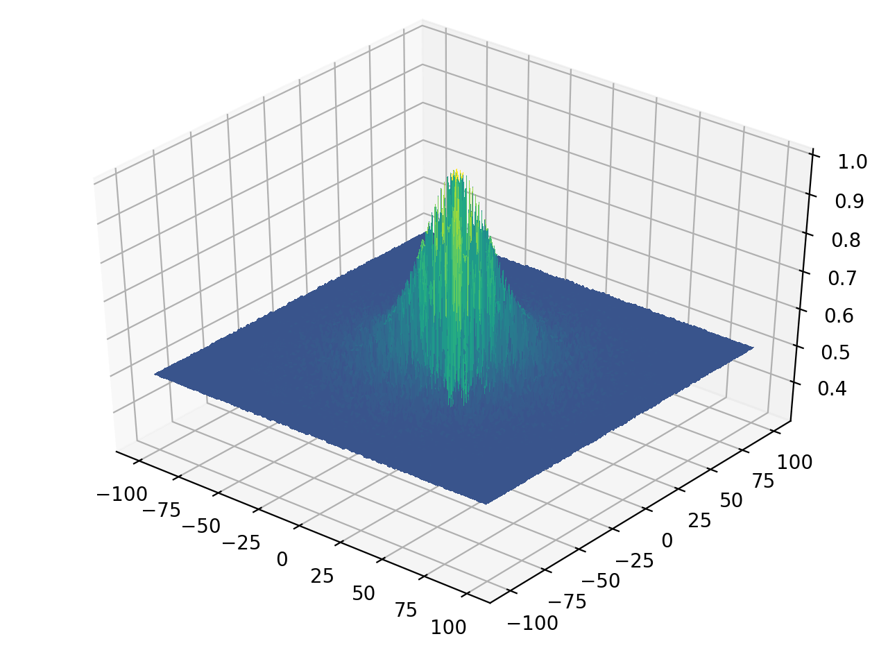
Schaffer function N.2
from landscapes.single_objective import schaffer_n2
| global minimum | bounds | usage |
|---|---|---|
| f(x=0, y=0) = 0 | -100 <= x, y <= 100 | schaffer_n2([x,y]) |
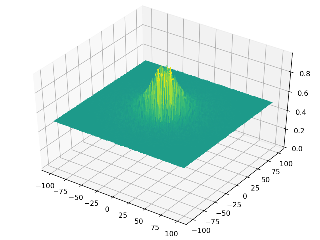
Schaffer function N.4
from landscapes.single_objective import schaffer_n4
| global minimum | bounds | usage |
|---|---|---|
| f(x=0, y=1.25313) = 0.292579 f(x=0, y=-1.25313) = 0.292579 |
-100 <= x, y <= 100 | schaffer_n4([x,y]) |
Sphere function
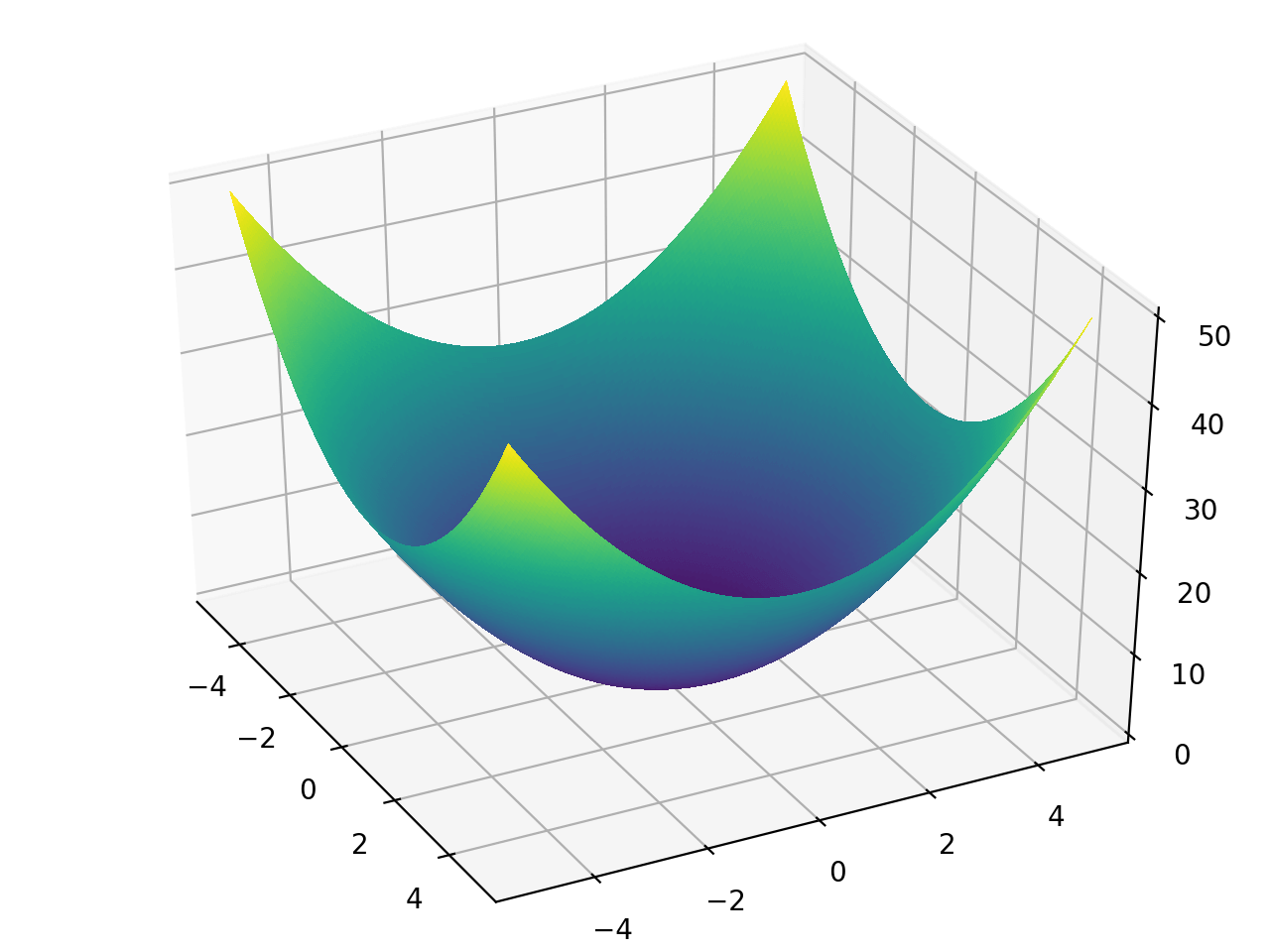
from landscapes.single_objective import sphere
| global minimum | bounds | usage |
|---|---|---|
| f([0,...,0]) = 0 | -inf <= x_i <= inf | sphere([x_1,...x_n]) |
Styblinski–Tang function
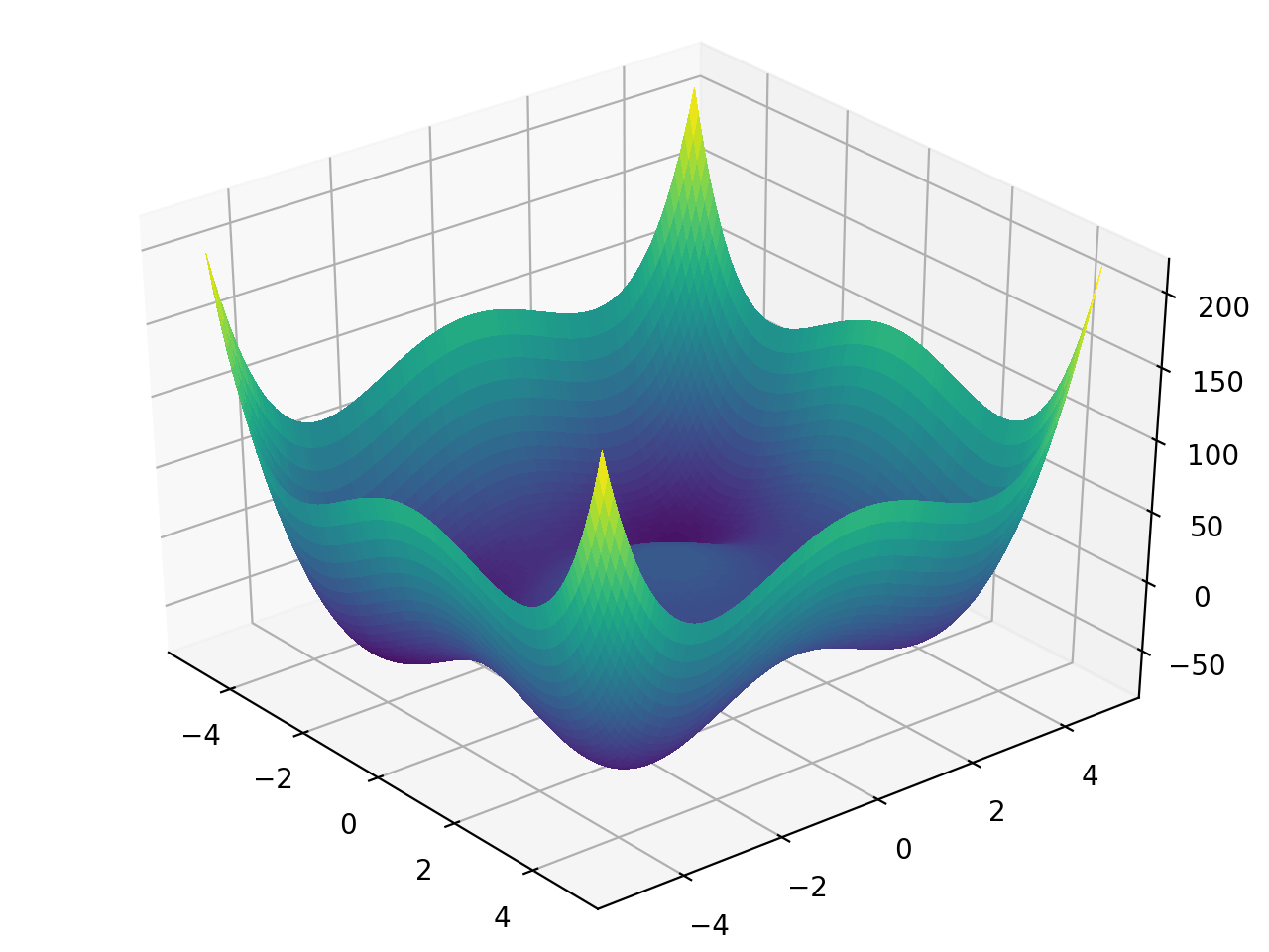
from landscapes.single_objective import styblinski_tang
| global minimum | bounds | usage |
|---|---|---|
| -39.16617n < f([-2.903534,...,-2.903534]) < -39.16616n | -5 <= x_i <= 5 | styblinski_tang([x_1,...x_n]) |
Three-hump camel function
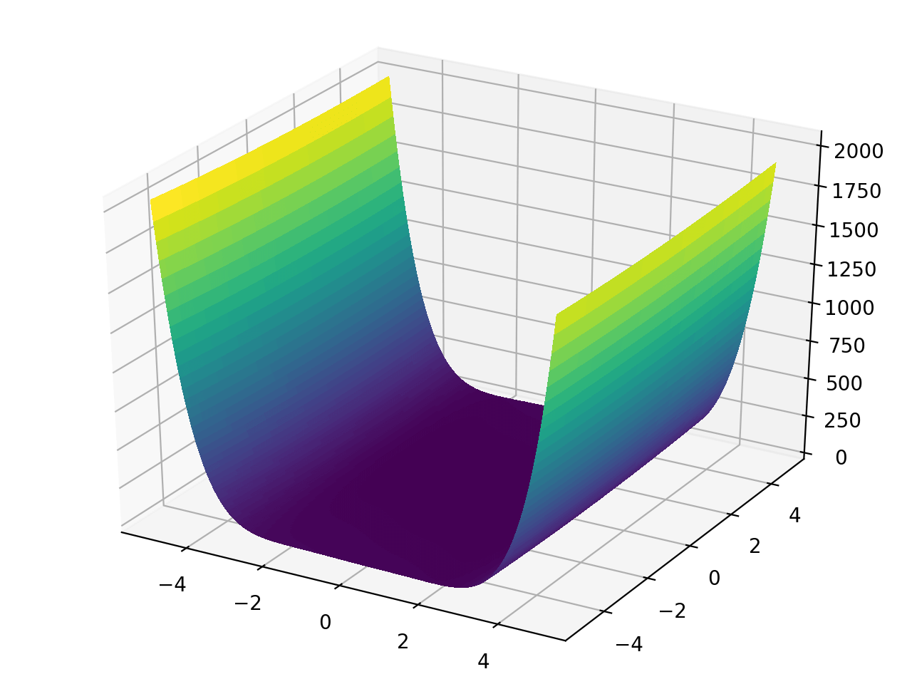
from landscapes.single_objective import camel_hump_3
| global minimum | bounds | usage |
|---|---|---|
| -f(x=0, y=0) = 0 | -5 <= x_i <= 5 | three_hump_camel([x,y]) |
Travelling salesman problem (TSP)
from landscapes.single_objective import tsp
There are several ways to use the TSP function within Landscapes, all of which involve specifying a list of tsp stops, and a distance function.
Example 1: Multi-dimensional list of points using Euclidean distance function
from landscapes.single_objective import tsp
from scipy.spatial import distance

np.random.seed(10)
pts = np.random.rand(5,3)
which will yield a list of three-dimensional points:
array([[0.77132064, 0.02075195, 0.63364823],
       [0.74880388, 0.49850701, 0.22479665],
       [0.19806286, 0.76053071, 0.16911084],
       [0.08833981, 0.68535982, 0.95339335],
       [0.00394827, 0.51219226, 0.81262096]])
Then, initialize the tsp function:
tsp_cost = tsp(distance.euclidean, close_loop=True).dist
To calculate the total travel distance, simply call the function with the list of points:
tsp_cost(pts)
>>> 3.2043803044101096
The flag close_loop simply specifies whether the distance between the first and last points should be calculated.
Example 2: Specifying points using Latitude and Longitude
Insead of multi-dimensional points in space, let's specify a list of locations based on longitude and latitude then calculate the distances using the inverse Vincenty's formulae which is available in the spatial package [here].
First let's import our Vincenty based distance function and wrap it for easier use.
from spatial import vincenty_inverse as vi

def vi_tsp(p1, p2):
    return vi(p1, p2).mi() # output distance in miles
Next, let's specify some locations. Here are some breweries in Cincinnati. Each row represents a [longitude, latitude].
pts = [
    [-84.508661, 39.110187],
    [-84.520021, 39.117219],
    [-84.514938, 39.113937],
    [-84.517401, 39.111322],
    [-84.476906, 39.128957]]
Again, initialize the tsp function:
tsp_cost = tsp(vi_tsp, close_loop=True).dist
And finally, calculate the travel distance:
tsp_cost(pts)
>>> 5.993331331465468
Example #3: Geospatial distances on a graph
In Example #2 we used Vincenty's inverse formulae which calculates the distance between two longitude and latitude pairs "as the crow flies". That's great for some situations, but in a city where we're limited by streets and sidewalks, it's a little less useful. Instead, what we want is the actual distance if we were going to walk or bike. This is the network distance and is only slighly more complex, but involves some additinal libraries.
First, import the dependencies:
import osmnx as ox
import networkx as nx
import pandas as pd
Next, load the brewery locations (available here) and prepare the Open Street Map (OSM) network graph.
pts_df = pd.read_csv('brewery_locations.csv')

# determine bounds for osm network
lats = locs_df['lat'].values
lngs = locs_df['lng'].values

bbox = [
    max(lats) + 0.1,
    min(lats) - 0.1,
    max(lngs) + 0.1,
    min(lngs) - 0.1]

# download osm street network
G = ox.graph_from_bbox(bbox[0], bbox[1], bbox[2], bbox[3], network_type='drive')
Downloading the osm graph might take a bit depending on internet speed. Next, let's create a new cost function that takes in two brewery names and returns the network distance in meters.
def osm_dist(n0, n1):
    p0 = pts_df[pts_df['name']==n0][['lat','lng']].values[0]
    p1 = pts_df[pts_df['name']==n1][['lat','lng']].values[0]

    p0_node = ox.get_nearest_node(G, p0)
    p1_node = ox.get_nearest_node(G, p1)

    dist_m = nx.shortest_path_length(G, p0_node, p1_node, weight='length')
    return dist_m
Again, specify the tsp cost function:
tsp_cost = tsp(osm_dist, close_loop=True).dist
And to get the network distance:
tsp_cost(locs_df['name'].values)
>>> 75950.73399999998
This translates to roughly 47 miles.
1 maintainer

Metadata
1 maintainer
Release files for landscapes 0.0.13
For a detailed explanation of source distributions (sdists) and built distributions (wheels), please see the package formats documentation.
Source distribution (sdist)
| File | Size | Uploaded | |
|---|---|---|---|
| landscapes-0.0.13.tar.gz | 21.7 kB | Details |
Built distribution (wheel)
| File | Interpreter | ABI | Platform | Reset |
|---|---|---|---|---|
| landscapes-0.0.13-py3-none-any.whl | Python 3 | none | any | Details |
Total release size: 37.5 kB
Release files / landscapes-0.0.13.tar.gz
| Download URL | landscapes-0.0.13.tar.gz |
|---|---|
| Size | 21.7 kB |
| Tags | Source |
|
SHA-256 checksum How to use checksums |
18a9e630e36a8d842b8df35fb740f892ac669493dd91386196a0eca0ca966c09
|
|
BLAKE2b-256 checksum How to use checksums |
696ce47f30d3ce3f986fb757164ff6a97829470c3989695fdcd59e362642a0d4
|
| Upload date | |
|
Uploaded using Trusted Publishing? What is trusted publishing? |
No |
| Uploaded via |
twine/6.2.0 CPython/3.14.2
|
Release files / landscapes-0.0.13-py3-none-any.whl
| Download URL | landscapes-0.0.13-py3-none-any.whl |
|---|---|
| Size | 15.8 kB |
| Tags | Python 3 |
|
SHA-256 checksum How to use checksums |
edd6699e7e34a14f173945af01c72940d113aa52ff4f666eb04160fa1bb60b83
|
|
BLAKE2b-256 checksum How to use checksums |
1b148f5ce59a6df0e0df118b764e15cd9caf9cb5785ccb8eceeefed1fdca6496
|
| Upload date | |
|
Uploaded using Trusted Publishing? What is trusted publishing? |
No |
| Uploaded via |
twine/6.2.0 CPython/3.14.2
|














