
FastLSQ
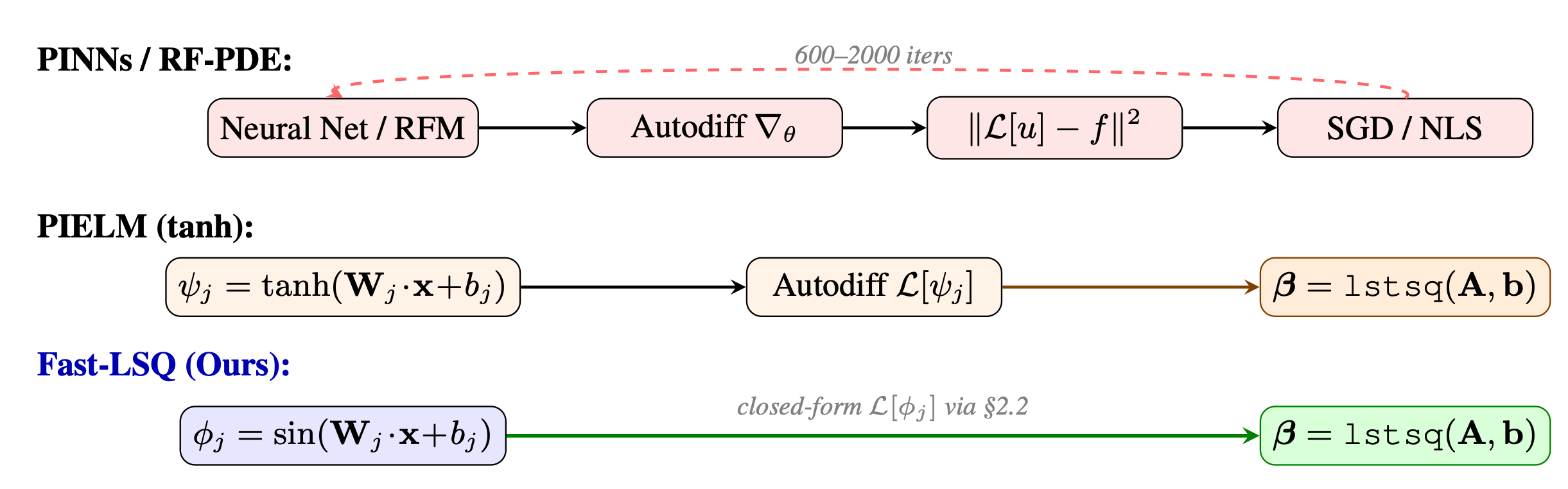
Solving PDEs in one shot via Fourier features with exact analytical derivatives.
FastLSQ is a lightweight PDE solver built around SinusoidalBasis, an
analytical derivative engine for random Fourier features. For sinusoidal
features phi_j(x) = sin(W_j . x + b_j), every derivative of every order
admits an exact closed-form expression -- no automatic differentiation needed.
Linear PDEs are solved in a single least-squares step. The random-feature system is typically rank-deficient, so the solve is routed through a backward-stable, auto-selected least-squares back-end (Cholesky fast-path -> Householder QR -> rank-revealing SVD) that runs on CPU, CUDA, or Apple-MPS. Nonlinear PDEs are solved via Newton-Raphson iteration with Tikhonov regularisation, 1/sqrt(N) feature normalisation, and continuation/homotopy.
Installation
pip install fastlsq
For development (includes testing and build tools):
git clone https://github.com/sulcantonin/FastLSQ.git
cd FastLSQ
pip install -e ".[dev]"
Quick start
Solve a linear PDE in one line
from fastlsq import solve_linear
from fastlsq.problems.linear import PoissonND

problem = PoissonND()
result = solve_linear(problem, scale=5.0)

u_fn = result["u_fn"]
print(f"Value error: {result['metrics']['val_err']:.2e}")
Solve a nonlinear PDE
from fastlsq import solve_nonlinear
from fastlsq.problems.nonlinear import NLPoisson2D

problem = NLPoisson2D()
result = solve_nonlinear(problem, max_iter=30)

print(f"Converged in {result['n_iters']} iterations")
print(f"Value error: {result['metrics']['val_err']:.2e}")
Choose a solver back-end and device
The linear solve is routed automatically, but solve_linear exposes the
back-end via method= (see How it works for the routing):
from fastlsq import solve_linear, set_device
from fastlsq.problems.linear import PoissonND

# "auto" (default) -- Cholesky fast-path -> QR -> rank-revealing SVD
# "qr"             -- Householder QR; SVD-grade accuracy at QR cost (full-rank A)
# "svd"            -- rank-revealing truncated SVD; the rank-deficient-safe reference
# "cholesky"       -- normal-equations Cholesky; fast, well-conditioned A only
# "rsvd"           -- randomized SVD, O(MNk), for strongly low-rank A
result = solve_linear(PoissonND(), scale=5.0, method="qr")

# Device selection (CPU / CUDA / Apple-MPS), or set FASTLSQ_DEVICE=cuda
set_device("cuda")   # the float64 default stays on CPU/CUDA; MPS is float32-only
Use the basis directly
import torch
from fastlsq.basis import SinusoidalBasis

basis = SinusoidalBasis.random(input_dim=2, n_features=1500, sigma=5.0)
x = torch.rand(5000, 2)

# Arbitrary mixed partial via multi-index
d2_dxdy = basis.derivative(x, alpha=(1, 1))

# Or use fast-path methods
H     = basis.evaluate(x)            # (5000, 1500)
dH    = basis.gradient(x)            # (5000, 2, 1500)
lap_H = basis.laplacian(x)           # (5000, 1500)
Compose PDE operators symbolically
import torch
from fastlsq.basis import SinusoidalBasis, Op

basis = SinusoidalBasis.random(input_dim=2, n_features=1500, sigma=5.0)
x = torch.rand(5000, 2)

# Coefficients can be scalars or nn.Parameter (for AdamW optimisation)
k, c = 10.0, 2.0
helmholtz = Op.laplacian(d=2) + k**2 * Op.identity(d=2)
A_pde = helmholtz.apply(basis, x)    # (5000, 1500)

wave = Op.partial(dim=2, order=2, d=3) - c**2 * Op.laplacian(d=3, dims=[0, 1])
Nonlocal operators (fractional Laplacian, convolution)
Every feature is a plane wave, so a Fourier multiplier m(ξ) acts diagonally
on the basis -- assembling it is a per-column rescale, exact, with no quadrature
and no discretisation of the (singular, nonlocal) kernel:
from fastlsq.basis import SinusoidalBasis, SymbolOperator, Op

basis = SinusoidalBasis.random(input_dim=2, n_features=1500, sigma=5.0)

frac = SymbolOperator.fractional_laplacian(s=0.75)   # (−Δ)^0.75
A    = frac.apply(basis, x)                          # (M, 1500), one rescale

# Mixes freely with differential terms
L = SymbolOperator.fractional_laplacian(0.5) + 3.0 * Op.identity(d=2)

# Convolution from the kernel's transform; s may be an nn.Parameter, so the
# fractional order itself can be recovered by gradient descent.
K = SymbolOperator.convolution(lambda W: torch.exp(-(W**2).sum(0, keepdim=True) / 12))
s=1 reproduces −Δ bit-exactly. Note this is the whole-space (restricted)
(−Δ)^s, not the spectral variant defined on a bounded domain -- the two differ
once the domain is bounded.
Integral equations (Fredholm, Volterra, separable kernels)
A separable kernel K(x,y) = Σ g_m(x) h_m(y) collapses the integral operator to
Σ_m g_m(x) ∫ h_m u, so acting on the basis needs only an R × N matrix of
inner products, computed once. A Fredholm equation of the second kind is then
one linear least squares like everything else:
from fastlsq import SeparableKernelOperator, fredholm_second_kind, degenerate_eigenvalues

# u(x) − λ ∫₀¹ x y u(y) dy = f(x)
K = SeparableKernelOperator([lambda x: x[:, 0]],      # g_m
                            [lambda y: y[:, 0]],      # h_m
                            lower=0.0, upper=1.0, d=1)

print(degenerate_eigenvalues(K, basis))    # λ where the equation is singular → 3.0
print(K.check_quadrature(basis))           # are the inner products resolved?

L = fredholm_second_kind(K, lam=0.5, d=1)
beta = solve_lstsq(L.apply(basis, x), f(x))
Second-kind equations need no boundary rows — the identity term makes them
well posed on its own. Integration over several axes at once (definite, running,
or mixed) is MultiIntegralOperator:
from fastlsq import MultiIntegralOperator

area = MultiIntegralOperator.definite([0, 1], [0, 0], [1, 1], d=2)   # ∫∫ over a box
memory = MultiIntegralOperator([0, 1], [0.0, 0.0], d=2, uppers=[1.0, None])  # definite × running
Ready-made problems with closed-form solutions live in fastlsq.problems and run
through solve_linear like the PDEs (PYTHONPATH=. python3 examples/integral_equations.py, 300 features, 2000 collocation points):
| Problem | rel L2 | grad rel L2 | boundary rows |
|---|---|---|---|
FredholmProductKernel(lam=0.5) |
5.5e-14 | 5.7e-12 | 0 |
FredholmProductKernel(lam=2.0) |
3.8e-13 | 3.9e-11 | 0 |
FredholmRank2Kernel(lam=0.4) |
9.1e-14 | 9.5e-12 | 0 |
VolterraSecondKind(lam=1.5) |
8.8e-13 | 1.0e-10 | 0 |
IntegroDifferentialODE(lam=4.0) |
6.2e-16 | 1.7e-14 | 1 |
Errors are against the closed-form solutions (degenerate-kernel theory for
the Fredholm cases, the equivalent ODE for the Volterra ones), not a reference
quadrature. Accuracy degrades gracefully toward the kernel's singular value --
for K = xy, whose only characteristic value is λ = 3, the error moves from
5.5e-14 at λ = 0.5 to 3.9e-12 at λ = 2.99.
Complex geometry without a mesh
A domain is any callable that is negative inside. Interior points come from
rejection sampling, boundary points from projection onto ψ = 0, and outward
normals from ∇ψ/‖∇ψ‖ -- which is exactly what Neumann and Robin conditions need:
from fastlsq.geometry import SDFDomain

dom = SDFDomain.annulus(0.3, 1.0)         # or .disk() .lshape() .flower() .tokamak()
x   = dom.sample(4000)                    # interior collocation
xb  = dom.sample_boundary(600)            # boundary collocation
B   = dom.neumann_rows(basis, xb)         # (M, N) block for ∂u/∂n = g

# Non-convex and multiply-connected domains are built, not meshed
plate = SDFDomain.disk(1.0) - SDFDomain.disk(0.2, center=(0.4, 0.0))
Built-in domains, as SDFDomain constructors or as bare ψ callables:
| Domain | SDFDomain |
Bare ψ |
Why it's there |
|---|---|---|---|
| Ball / disk | .ball(), .disk() |
sdf_ball, sdf_disk |
Exact SDF, any dimension; the §2.7 unit disk |
| Axis-aligned box | .box(lo, hi) |
sdf_box |
Exact inside and out; the CSG building block |
| Annulus / shell | .annulus(r_in, r_out) |
sdf_annulus |
Multiply-connected — an interior boundary whose outward normal points toward the centre |
| L-shape | .lshape(size, cut) |
sdf_lshape |
Reentrant corner, the standard non-convex stress case (r^{2/3} solution singularity) |
| Flower | .flower(R, a, k) |
sdf_flower |
Smooth non-convex, and deliberately not a distance function (‖∇ψ‖ spans 1–10) — the case that separates a correct projection from a naive one |
| Polygon | — | sdf_polygon(verts) |
Exact for any simple polygon; the escape hatch for a cross-section known only as a curve (measured, CAD, traced) |
| Tokamak | .tokamak() |
sdf_tokamak |
D-shaped Miller poloidal cross-section, via sdf_polygon |
Any ψ of your own works too — it only has to be negative inside. Combine them
with the CSG helpers, which are also available as plain functions:
| Set operation | Operator | Function |
|---|---|---|
Union A ∪ B |
A | B |
sdf_union(a, b) |
Intersection A ∩ B |
A & B |
sdf_intersection(a, b) |
Difference A \ B |
A - B |
sdf_difference(a, b) |
| Complement | — | sdf_complement(a) |
CSG results are valid implicit functions (correct sign everywhere) but not
generally exact distance functions — min/max of two exact SDFs over- or
under-estimates distance near the seam. Nothing here depends on exactness:
sampling uses only the sign, and project_to_boundary normalises by ‖∇ψ‖².
Vector-valued solutions
solve_linear / solve_nonlinear support vector-valued u: ℝᵈ → ℝᵏ for
coupled systems (elasticity, Stokes, Maxwell vector potential, …) and for
decoupled multi-output problems sharing one basis. The math is unchanged; the
solver just allocates beta with shape (N, k) so that solver.predict(x)
returns shape (M, k) directly.
A problem opts in by setting self.n_outputs = k and assembling its operator
in block-stacked form A ∈ ℝ^{Mk × Nk}, b ∈ ℝ^{Mk × 1}. The helper
block_concat removes the manual torch.cat bookkeeping:
import torch
from fastlsq import solve_linear, block_concat

class Stokes2D:
    n_outputs = 3        # (u, v, p)
    dim = 2
    name = "Stokes 2D"
    # ... exact, exact_grad, get_train_data, get_test_points ...

    def build(self, slv, x, bcs, f):
        basis = slv.basis
        cache = basis.cache(x)
        dx = basis.derivative(x, (1, 0), cache=cache)
        dy = basis.derivative(x, (0, 1), cache=cache)
        lap = basis.laplacian(x, cache=cache)

        # Rows = equations (mom_x, mom_y, continuity);
        # columns = coefficient blocks (u, v, p)
        A = block_concat([
            [-lap,  None,  dx  ],   # -Δu + ∂p/∂x = f_x
            [ None, -lap,  dy  ],   # -Δv + ∂p/∂y = f_y
            [ dx,   dy,    None],   #  ∂u/∂x + ∂v/∂y = 0
        ])
        b = block_concat([[f[:, 0:1]], [f[:, 1:2]], [torch.zeros_like(f[:, 0:1])]])
        # ... add BC blocks the same way ...
        return A, b

result = solve_linear(Stokes2D(), scale=5.0)
u = result["u_fn"](x_test)        # shape (M, 3): columns are (u, v, p)
Partial derivatives for a vector u
The basis-level operators (basis.derivative, basis.gradient,
basis.laplacian, DiffOperator.apply) all return shape (M, N) regardless
of how many components u has — vector-ness only enters when you contract
with beta:
# Full Jacobian, then slice (M, d, k) -> per (component, dim)
u, J = solver.predict_with_grad(x)   # J shape (M, d, k); J[:, j, c] = ∂u_c/∂x_j

# Single operator on a single component
D_y = solver.basis.derivative(x, alpha=(0, 1))   # (M, N): ∂φ/∂y
du0_dy = D_y @ solver.beta[:, 0:1]               # ∂u_0/∂y

# Symbolic operator, all components at once
from fastlsq import Op
yy = Op.partial(dim=1, order=2, d=2)
A  = yy.apply(solver.basis, x)                   # (M, N)
u_yy = A @ solver.beta                           # (M, k): ∂²u/∂y² per component
Scalar problems are untouched: n_outputs defaults to 1, solver.beta keeps
shape (N, 1), and predict_with_grad returns gradient shape (M, d) for
backward compatibility (the trailing component axis is squeezed when k=1). The
Stokes2D sketch above and tests/test_block.py -- a
runnable block_concat + unpack_beta solve that recovers both components of a
k=2 system -- are the reference for the block-stacked vector path.
Plot solutions
from fastlsq.plotting import plot_solution_2d_contour, plot_convergence

plot_solution_2d_contour(result["solver"], problem, save_path="solution.png")
plot_convergence(result["history"], problem_name=problem.name, save_path="convergence.png")
Benchmarks
# Linear PDE benchmark (Fast-LSQ vs PIELM)
python examples/run_linear.py

# Nonlinear PDE benchmark (Newton-Raphson)
python examples/run_nonlinear.py

# Learnable Helmholtz wavenumber (nn.Parameter + AdamW)
python examples/learnable_helmholtz.py
Inverse problems
The analytical derivatives enable gradients through the pre-factored solve, making inverse problems tractable. Example: recovering 4 anisotropic Gaussian heat sources (24 parameters) from 4 sparse sensors. The heat equation is solved in space-time; L-BFGS-B optimises source positions and shapes to match sensor time-series. (Click image for animation.)
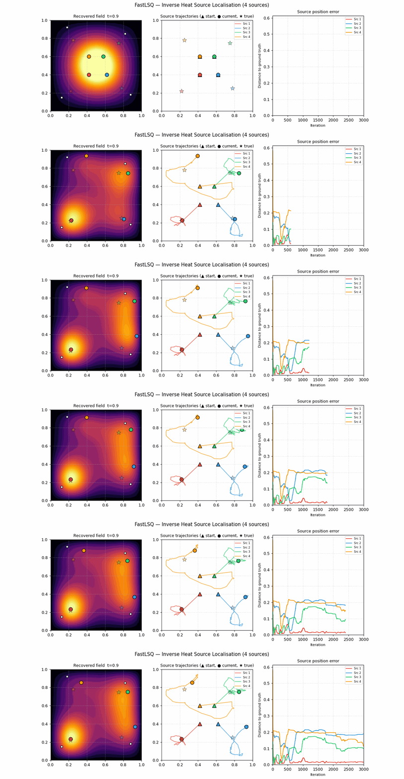
python examples/inverse_heat_source.py
Core architecture
The framework is built around SinusoidalBasis -- the analytical
derivative engine:
| Class | Purpose |
|---|---|
SinusoidalBasis |
Evaluates basis functions and arbitrary-order derivatives in O(1) via the cyclic identity |
BasisCache |
Pre-computes sin(Z)/cos(Z) once, reuses across multiple derivative evaluations |
DiffOperator / Op |
Symbolic linear differential operators that compose via +, -, scalar *; coefficients can be nn.Parameter for learnable PDEs |
IntegralOperator / IntegroDifferentialOperator |
Closed-form single-axis definite / running (Volterra) integrals, including order=n iterated integrals ∫_lo^x (x−t)^{n−1}/(n−1)! φ dt; compose with Op into one integro-differential design matrix |
MultiIntegralOperator |
Closed-form integration over several axes at once, each independently definite or Volterra -- area/volume functionals and mixed "definite in space, running in time" memory terms. The plane wave factorises over axes, so it is a product of the same stable one-axis factors |
SeparableKernelOperator |
Separable (degenerate) kernels K(x,y) = Σ g_m(x) h_m(y), assembled as a rank-R product G @ C with the inner products C precomputed once. With fredholm_second_kind this makes u − λ∫K u = f one linear least squares |
SymbolOperator |
Fourier-multiplier (nonlocal) operators L e^{iξ·x} = m(ξ) e^{iξ·x}. Features are plane waves, so the symbol acts diagonally -- a per-column rescale, exact, no quadrature. Ships fractional_laplacian(s) (with learnable s), riesz_potential, riesz_transform, convolution(k̂) |
GaussianWindowedBasis / ProjectionOperator |
Windowed-Fourier (Gabor) basis + closed-form projection (Radon) operator ∫ f δ(c·z−u) dz for tomographic / line-integral inverse problems; quadrature-free and differentiable in the optics c |
AugmentedBasis / PolynomialColumns |
Widens a basis with explicit 1, x, x², … columns carrying exact operator images, to pin integration constants and DC modes that leave the sinusoidal family. Transparent to every operator |
SDFDomain + sample_sdf / project_to_boundary / outward_normal |
Membership-oracle geometry: give any ψ(x) negative inside and get interior points, boundary points and outward normals -- no mesh. CSG composition via |, &, -; built-ins include disk, annulus, L-shape, flower, polygon and a tokamak cross-section |
FeatureBasis |
Adapter for non-sinusoidal solvers (e.g. PIELM with tanh) |
FastLSQSolver |
Manages feature blocks; exposes .basis for all derivative computations |
LearnableFastLSQ |
Differentiable solver with learnable bandwidth via reparameterisation trick |
block_concat, pack_beta, unpack_beta |
Block-structured assembly helpers for vector-valued u (coupled systems). solver.beta has shape (N, k); scalar problems are the k=1 case |
solve_lstsq |
Multi-back-end least-squares solve (auto/qr/svd/cholesky/rsvd); rank-revealing by default for the rank-deficient feature matrix |
resolve_device / set_device / get_device |
CPU / CUDA / Apple-MPS selection, dtype-aware (MPS is float32-only; factorizations fall back to CPU) |
How it works
-
Basis construction. Given collocation points x, construct a
SinusoidalBasiswith random weights W and biases b. The collocation counts default to scale with the feature count (n_pde = max(3000, 3 * n_blocks * hidden_size),n_bc = max(800, n_pde // 5)). -
Analytical derivatives. Exploit the cyclic derivative identity: the n-th derivative of sin(z) cycles through {sin, cos, -sin, -cos} with monomial weight prefactors. Any mixed partial
D^alpha phi_j(x)is computed in O(1) -- no computational graph, no automatic differentiation. -
PDE assembly. Define the differential operator symbolically with
Op(e.g.Op.laplacian(d=2)) and apply it to the basis to get the system matrixA. -
Linear solve. Solve
A beta = bin the least-squares sense. The random-feature matrixAis typically rank-deficient (near-duplicate columns), so the defaultmethod="auto"starts from a Cholesky fast-path (guarded by a cheap conditioning probe), falls back to backward-stable Householder QR, and resorts to a rank-revealing SVD only if the QR solution blows up. A Tikhonov ridgemuenters via the[A; sqrt(mu) I]augmentation, not the condition-squaring normal equations. -
Newton iteration (nonlinear). Linearise the PDE residual, solve
J delta_beta = -Rwith backtracking line search, and repeat.
Adding your own PDE
Define a problem class and use solver.basis to build the linear system:
import torch, numpy as np
from fastlsq import solve_linear, Op
from fastlsq.geometry import sample_box, sample_boundary_box

class MyPoisson2D:
    def __init__(self):
        self.name = "My Poisson"
        self.dim = 2
        self.pde_op = -Op.laplacian(d=2)

    def exact(self, x):
        return torch.sin(np.pi * x[:, 0:1]) * torch.sin(np.pi * x[:, 1:2])

    def exact_grad(self, x):
        sx, cx = torch.sin(np.pi * x[:, 0:1]), torch.cos(np.pi * x[:, 0:1])
        sy, cy = torch.sin(np.pi * x[:, 1:2]), torch.cos(np.pi * x[:, 1:2])
        return torch.cat([np.pi * cx * sy, np.pi * sx * cy], dim=1)

    def source(self, x):
        return 2 * np.pi**2 * self.exact(x)

    def get_train_data(self, n_pde=5000, n_bc=1000):
        x_pde = sample_box(n_pde, self.dim)
        f_pde = self.source(x_pde)
        x_bc = sample_boundary_box(n_bc, self.dim)
        u_bc = self.exact(x_bc)
        return x_pde, [(x_bc, u_bc)], f_pde

    def build(self, solver, x_pde, bcs, f_pde):
        basis = solver.basis
        cache = basis.cache(x_pde)
        A_pde = self.pde_op.apply(basis, x_pde, cache=cache)
        As, bs = [A_pde], [f_pde]
        for (x_bc, u_bc) in bcs:
            As.append(100.0 * basis.evaluate(x_bc))
            bs.append(100.0 * u_bc)
        return torch.cat(As), torch.cat(bs)

    def get_test_points(self, n=5000):
        return sample_box(n, self.dim)

result = solve_linear(MyPoisson2D(), scale=5.0)
See examples/add_your_own_pde.py for the complete tutorial.
Features
- Analytical derivative engine:
SinusoidalBasiscomputes arbitrary-order derivatives exactly in O(1) -- the foundation of the entire framework - Symbolic PDE operators: Compose differential operators with
Op(Laplacian, wave, Helmholtz, biharmonic, custom) via intuitive arithmetic; coefficients can benn.Parameterfor AdamW optimisation - Closed-form integral operators:
IntegralOperator(single-axis definite / Volterra integrals) composes withOpinto one integro-differential least-squares block. The integral class now also includes the projection (Radon) operator (ProjectionOperatoron aGaussianWindowedBasis) -- quadrature-free∫ f δ(c·z−u) dzline/hyperplane integrals for tomographic inverse problems, differentiable in the opticscfor experiment design - Integral equations: Separable (degenerate) kernels
K = Σ g_m(x) h_m(y)assemble as a rank-Rproduct with inner products precomputed once, so a Fredholm equation of the second kindu − λ∫K u = fis a single linear least squares needing no boundary rows.degenerate_eigenvaluesreports theλat which the equation is singular andcheck_quadraturewhether the inner products are resolved -- both otherwise-silent failure modes.MultiIntegralOperatorintegrates over several axes at once, each independently definite or Volterra - Nonlocal / Fourier-symbol operators:
SymbolOperatorassembles any multiplierm(ξ)as a per-column rescale -- exact, quadrature-free, and the same cost as the Laplacian. Covers the fractional Laplacian(−Δ)^s(with a learnable orders), Riesz potentials and transforms, and convolutionk * ufrom the kernel transformk̂. Operators whose kernels are singular and nonlocal -- dense, ill-conditioned matrices for FEM/FD -- are diagonal here - Vector-valued solutions: First-class support for u: ℝᵈ → ℝᵏ (elasticity, Stokes, Maxwell). Problems declare
n_outputs = k;block_concatassembles coupled block systems;solver.predict(x)returns shape(M, k). Scalar problems are thek=1case - Augmentation columns:
AugmentedBasis+PolynomialColumnswiden the basis with exact1, x, x², …columns to pin integration constants and DC modes that leave the sinusoidal family -- transparent to every operator - High-level API: Solve PDEs in one line with
solve_linear()andsolve_nonlinear() - Robust linear solver: Pluggable least-squares back-ends; the default
autoroutes Cholesky -> QR -> SVD, and backward-stable QR delivers SVD-grade accuracy at QR cost on the rank-deficient random-feature system - Learnable bandwidth:
LearnableFastLSQoptimises the bandwidth (scalar or anisotropic) via reparameterisation - Learnable PDE coefficients: Plug
nn.ParameterintoOp(e.g. Helmholtz wavenumberk) and optimise via AdamW; gradients flow through the prebuilt linear solve - Auto-tuning: Automatic scale selection via grid search
- Device support: CPU / CUDA / Apple-MPS via
set_device()or theFASTLSQ_DEVICEenv var, dtype-aware (the float64 high-accuracy path stays on CPU/CUDA) - Adaptive collocation:
n_pde/n_bcdefault to feature-count-scaled values, overridable per solve - Built-in plotting: Solution visualization, convergence plots, spectral sensitivity
- Geometry samplers: Box, ball, sphere, interval, custom samplers
- Meshless complex geometry:
SDFDomaintakes any membership oracleψ(x)(negative inside) and supplies interior points, boundary points and outward normals∇ψ/‖∇ψ‖for Neumann/Robin conditions. CSG composition (|,&,-) builds non-convex and multiply-connected domains; built-ins include disk, annulus, L-shape, flower, arbitrary polygon, and a D-shaped tokamak poloidal cross-section - Diagnostics: Problem validation, conditioning checks, error detection
- Export utilities: NumPy conversion, checkpoint saving/loading
- PyTorch Lightning: Integration for training loops
- 20+ benchmark problems: Linear, nonlinear, and regression-mode PDEs
Paper
The full preprint is available on arXiv
Citing this work
If you use FastLSQ in your research, please cite:
@misc{sulc2026fastlsqframeworkoneshotpde,
      title={FastLSQ: A Framework for One-Shot PDE Solving},
      author={Antonin Sulc},
      year={2026},
      eprint={2602.10541},
      archivePrefix={arXiv},
      primaryClass={math.NA},
      url={https://arxiv.org/abs/2602.10541},
}
License
This project is licensed under the MIT License -- see LICENSE for details.
1 maintainer

Download files
Download the file for your platform. If you're not sure which to choose, learn more about installing packages.
Source Distribution
Built Distribution
Filter files by name, interpreter, ABI, and platform.
If you're not sure about the file name format, learn more about wheel file names.
Copy a direct link to the current filters
File details
Details for the file fastlsq-0.6.0.tar.gz.
File metadata
- Download URL: fastlsq-0.6.0.tar.gz
- Upload date:
- Size: 331.3 kB
- Tags: Source
- Uploaded using Trusted Publishing? No
- Uploaded via:
twine/6.2.0 CPython/3.10.12
File hashes
| Algorithm | Hash digest | |
|---|---|---|
| SHA256 |
8468d5304b8564eaf24c23ab44217ab02d99f037092b74d7c66ecfe6a6ad98d5
|
|
| MD5 |
b74092f5b1639d5bd55395268158b8f6
|
|
| BLAKE2b-256 |
883528deaca795f7f3d19a7d9736909c29fd04cf3d614ae953ff95442da33cfb
|
File details
Details for the file fastlsq-0.6.0-py3-none-any.whl.
File metadata
- Download URL: fastlsq-0.6.0-py3-none-any.whl
- Upload date:
- Size: 112.5 kB
- Tags: Python 3
- Uploaded using Trusted Publishing? No
- Uploaded via:
twine/6.2.0 CPython/3.10.12
File hashes
| Algorithm | Hash digest | |
|---|---|---|
| SHA256 |
edb33936b8602106aad9faac7fd237a91c5e859f32390b6402446e340dc2478c
|
|
| MD5 |
8892db3ca0cb3562347b0399ee6e2251
|
|
| BLAKE2b-256 |
219346cdcee2e75f16346ae2e1d99b2e3a3902c90fe12b838eff81006b31d19d
|







