A python package for clustering and summarizing graphs of texts.

Project description
Graph Clustering and Summarizing
Introduction
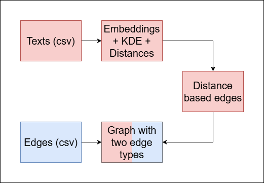
We aim to improve the quality of a multi-document summary, given the connections between the texts (via shared authors, institution, subject etc.). Our method is as follows:
- Calculate the direct distances between the texts in the graph.
- Build a new graph with two edge types:
- Blue edges: represent the original connections given.
- Red edges: represent similarity between texts.
- Cluster the multi color edged graph.
- Summarize each cluster.
- Evaluate the summarization of each cluster.
Our python package contains a full pipeline that performs the above operations (1-5), or alternatively perform specific operations individually.
Table of Contents
Installation
In a clean environment, simply type
pip install GraphClusterer
to download our python package, or alternatively clone this repository if you wish to manually tune the pipeline (recommended).
There is one difference between the usage of the package compared to the clone repository, which is a change in the .env file that is required for the repository, compared to the inclusion of the API keys needed as strings in the config.json file when using the package (see example in Quick tour).
Running example
There are two ways to run and use our project.
- using the python package (GraphClusterer)
- using a cloned version of this repository
|-- vertices.csv
|-- edges.csv
|-- config.json
|-- distance_matrix.pkl (optional)
|-- .env (required for the second case)
`-- main.py
And after running the code, the following directories will be added:
|-- data
|   `-- clusteder_graphs
|       `-- name.gpickle
|
|-- Results
|   |-- Summaries
|   |   `-- name
|   |       |-- title_1.txt
|   |       |-- ...
|   |       `-- title_n.txt
|   |
|   |-- starry
|   |   |-- name.csv
|   |   `-- name_titles.csv
|   |
|   |-- plots
|   |   `-- name.png
|   |
|   `-- html
|       `-- name.html
|
`-- metrics.json
If distance_matrix is provided and valid (see file formats below), the following directories will be added to data after running:
data
|-- embeddings
|   `-- vertices_file_name_embeddings.pkl
|
`-- kde_values
    `-- name.pkl
Which cache the embedding vectors for each sentence, and the KDE values for filtering (NEED TO FULLY INTEGRATE MANUAL FILTERING INTO THE PIPELINE).
File formats
main.py
Here's an example script for the main file in the first case usage (the python package). If you intend on using the cloned repository, you can use the main.py file here.
from GraphClusterer.one_to_rule_them_all import the_almighty_function  # make the main function available.
from GraphClusterer.main import load_params, get_distance_matrix
import pandas as pd


if __name__ == '__main__':
    params = load_params('config.json')

    # Set the parameters for the pipeline.
    pipeline_kwargs = {
        'graph_kwargs': params['graph_kwargs'],
        'clustering_kwargs': params['clustering_kwargs'],
        'draw_kwargs': params['draw_kwargs'],
        'print_info': params['print_info'],
        'iteration_num': params['iteration_num'],
        'vertices': pd.read_csv(params['vertices_path']),
        'edges': pd.read_csv(params['edges_path']),
        'distance_matrix': get_distance_matrix(params['distance_matrix_path']),
        'name': params['name'],
        'key': params['cohere_key'],
        'llama_key': params['llama_key']
    }

    if params["allow_user_prompt"]:  # If the user prompt is allowed.
        user_aspects = input("Enter the aspects you want to focus on, separated by commas: ").split(",")
        pipeline_kwargs['aspects'] = user_aspects

    # Run the pipeline.
    the_almighty_function(pipeline_kwargs)
config.json
The config.json file requires core elements, and additional keys when using the python package, in order to avoid the usage of a .env file.
{
  "graph_kwargs": {
    "size": 2000,
    "K": 5,
    "color": "#1f78b4"
  },

  "clustering_kwargs": {
    "method": "louvain",
    "resolution": 0.5,
    "save": true
  },

  "draw_kwargs": {
    "save": true,
    "method": "louvain",
    "shown_percentage": 0.3
  },

  "name": "clock",
  "vertices_path": "clock_nodes.csv",
  "edges_path": "clock_edges.csv",
  "distance_matrix_path": "optional path to distance_matrix.pkl",

  "iteration_num": 1,
  "print_info": true,
  "cohere_key": "your Cohere API key here",
  "llama_key": "your Llama API key here"
}
.env
When using the cloned repository, you must have a .env file in the same working directory as main.py.
COHERE_API_KEY="your Cohere API key here"
REPLICATE_API_TOKEN="your Llama API key here"
vertices.csv
The pipeline expects a vertices file with the following structure for each line (text can be empty).
id |
abstract (includes the text to summarize) |
additional attributes (e.g. color, language, shape etc. Used for debugs and plotting. Each attribute in its own column) |
|---|---|---|
| vertex_1_id | vertex_1_abstract_text | vertex_1_attributes |
edges.csv
The pipeline expects a file containing the original edges (for distance-based edges see here). Each edge (row in the file) should have either 2 or 3 columns (if 3, all rows need to have 3 columns).
- The 2 column case occurs when only textual vertices are introduced in the graph.
- The 3 column case occurs when there are additional vertices without text in the edges file. In that case, the new vertices are added to the graph with their specified type (in the third column).
distance_matrix.pkl
The distance matrix needs to be an array of size NxN, where N is the number of textual vertices (rows in vertices.csv). If provided, the distance matrix is used to add a second type of edges (red edges).
Quick tour
To immediately use our package, you only need to use two functions.
In order to use the package (or cloned repository) you need to prepare a configuration file in advanced (see config.json).
There are two use cases:
- cloned repository: you also need to have a
.envfile in the same directory asmain.py, in which the API keys for llama and cohere are kept like the example here:
COHERE_API_KEY=[your API key for cohere (string format)]
REPLICATE_API_TOKEN=[your API token for llama (string format)]
- python package: you also need to include the following arguments in your
config.jsonfile:'cohere_key': [your API key for cohere (string format)], 'llama_key': [your API key for llama (string format)]
In both cases, your main.py code should be like:
params = load_params(config_path)
# Set the parameters for the pipeline.
pipeline_kwargs = {
   'graph_kwargs': params['graph_kwargs'],
   'clustering_kwargs': params['clustering_kwargs'],
   'draw_kwargs': params['draw_kwargs'],
   'print_info': params['print_info'],
   'iteration_num': params['iteration_num'],
   'vertices': pd.read_csv(params['vertices_path']),
   'edges': pd.read_csv(params['edges_path']),
   'distance_matrix': get_distance_matrix(params['distance_matrix_path']),
   'name': params['name'],
    }

# Run the pipeline.
one_to_rule_them_all.the_almighty_function(pipeline_kwargs)
Alternatively, you can manually perform each sub-task in our pipeline using the following functions:
- Create the graph with two edge colors:
functions.make_graph(**graph_kwargs) - Cluster the graph:
functions.cluster_graph(**clustering_kwargs) - Summarize each cluster:
summarize.summarize_per_color(**kwargs)(need to divide the graph into clusters and input a list of subgraphs) - Evaluate the clusters and summaries: several functions in the
evaluatemodule (see here)
You can also use the old versions and follow these instructions:
Case 1
In this case you can skip the graph processing part, and go straight to the clustering part. The prepared graph needs to include the followings:
- vertex attribute called 'content', whose value is the textual data of the vertex.
- (optional) vertex attribute called 'shape', in order to distinguish between texts in different languages (for now, this case deals with each language individually).
Case 2
In this case, we need to create the graph first.
- The csv containing vertex data has to be named '
{dataset name}_papers.csv', and has to contain at least an ID column and 'abstract' column. The ID column values are used to identify texts, and the 'abstract' column should contain the texts. - The csv containing edges has to be named '
{dataset name}_graph.csv' and have 2 columns by default, and each of its rows has to contain at least one identifiable text that appears in the vertex data file. In case the other element is not identifiable, a new vertex will be created, with a different type and no content. - Rows with 3 or more elements will be dealt as a clique.
Secondly, calculation of distances between texts are required. For that we firstly have to convert the texts to sets of embedding vectors.
We do that in '2_embed_abstracts.py' using the sentence-transformers package, refer to each text as a set of sentence embeddings, and calculate 'energy distance' between two texts (two sets of vectors) in 'calc_energy.py'.
In order to successfully estimate the distance between two texts, we filter sentences that interrupt the procedure (in our case, we prefer to filter out the most common sentences, as well as the rarest sentences). We do that by combining all of the sentences' embeddings in the dataset into one list, order the items according to their frequencies, and filtering least_cutoff_percentage embeddings from the least common sentences. Similarly, we filter most_cutoff_percentage embeddings from the most common sentences. Both cutoff parameters are optimized for each dataset given.
After filtering out the irrelevant embeddings, we compute the distances between each pair of texts using 'energy distance':
def compute_energy_distance_matrix(ds_name, least_cutoff_percentage, most_cutoff_percentage):
Where:
ds_name: The name of the dataset.least_cutoff_percentage: The percentage of data to filter among rare sentences.most_cutoff_percentage: The percentage of data to filter among frequent sentences. We then calculate the energy distance between each pair of embeddings using the usingdcorpackage.
Returns: The energy distance matrix for the matched embedding.
You can then run the graph creating part of our pipeline in 'functions.py':
def make_graph(name, **kwargs):
Where:
name: The name of the dataset.**kwargs: A dictionary of values to manually configure the graph creation. Here is an example dictionary:
graph_kwargs = {
        'size': 2000,
        'color': '#1f78b4',
        'K': 5,
    }
where:
k: The number of neighbors to account for in the distance based edges.color: The default vertex color (needed in order to plot the final vertex partition).size: The default vertex size (needed in order to plot the final vertex partition).
Returns: Processed graph (networkx.Graph object)
Clustering
After processing/creating the graph of texts (and keywords), we cluster the graph using the Louvain method with the implementation embedded in the networkx module.
In case the graph consists of keyword vertices, and not exclusively texts, the other vertices are included in the clustering part of our pipeline, but ignored from then on.
The clustering is also done in the 'function.py' source file. In addition to return the partition, our method also assigns each vertex with a color, as a way to map the vertices to clusters later on.
def cluster_graph(G, name, **kwargs):
Where:
G: The processed/given graph.name: The name of the dataset.**kwargs: A dictionary of values to manually configure the clustering process. Here is an example dictionary:
clustering_kwargs = {
        'save': True,
        'resolution': res,
        'weight': weight,
        'K': K
    }
Where:
save: A flag indicating whether to save the clustered graph as a '.gpickle' format or not.weight: The assigned weight for distance based edges.k: The number of neighbors to account for in the distance based edges.
Returns: $\mathcal{P}$ a partition of vertices from G into communities.
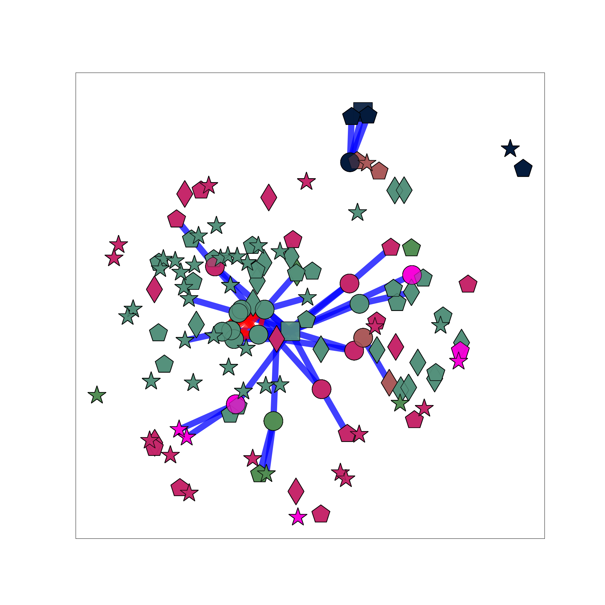
Example for the clustering:
Summarization
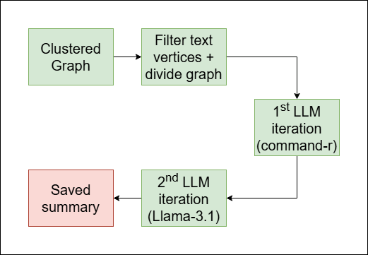
As mentioned in the introduction section, the main goal of our pipeline is to summarize clusters of vertices, rather than the full graph. To achieve that we perform the following steps:
-
Cluster the graph (see clustering).
-
Divide the graph according to the clusters (done in
filter_by_color()). -
Summarize each cluster individually. In this step, each time we are given a subgraph of only the cluster. Firstly we filter out non-textual vertices, then we access the texts and save them in a list, and then we send the list with a prompt to two iterations of LLM generation:
command-r: in this iteration, we generate a draft of the final summary.llama-3.1: in this iteration, we refine the summary and enrich its language.
And a third iteration generates a title for the summary (also made with
llama-3.1).
The full summarization process happen in summarize_per_color():
def summarize_per_color(subgraphs, name):
Where:
subgraphs: A list of subgraphs, each belong to a different cluster (see step 2).name: The name of the dataset.
The function fetches the texts from the vertices in the subgraph, send them to the above 3 iterations of LLM generation, and saves the summaries for each cluster as a '.txt' file in a folder named name.
Example of a summary:
Biomass-derived carbons (BDCs) and their composites with conductive materials, such as metals, metal sulfides, carbon nanotubes,
and reduced graphene oxide, are used to enhance the performance of supercapacitors. By combining BDCs with conductive additives,
researchers aim to improve conductivity, charge/discharge capabilities, and specific surface area, resulting in higher specific
capacitance values. This approach integrates the benefits of electrochemical double-layer capacitors (EDLCs) and pseudocapacitors,
leading to enhanced energy density. Layered double hydroxides (LDHs), synthetic two-dimensional nano-structured anionic clays, are
also explored as hosts for Azo-compounds to create nano-hybrid materials. Intercalating large anionic pigments like phenyl azobenzoic
sodium salt into Zn-Al LDH increases the interlayer spacing significantly, and the resulting nano-hybrid material is used as a filler
for polyvinyl alcohol (PVA) to form nano-composites that exhibit improved thermal stability compared to pure PVA.
Evaluation
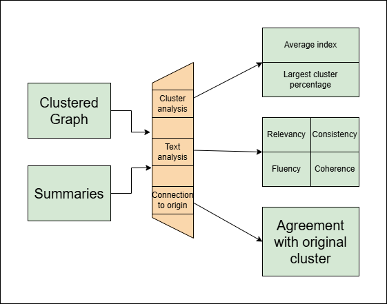
In the evaluation section, we execute a series of tests in order to assess the quality of:
- The clustering.
- The summaries (as text documents).
- The consistency between a summary and its origin.
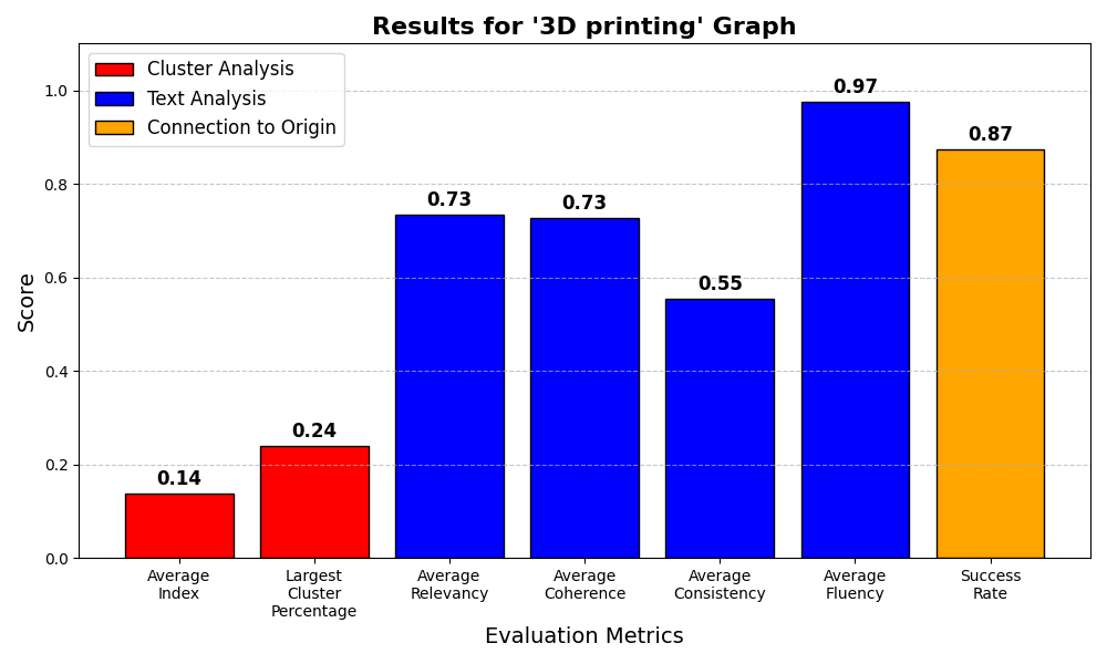
Clustering scores
The clustering scores evaluate how good the clustering partitioned the graph. For that we used two metrics (one is irrelevant if the graph is given by the user and not created by our 'make_graph()' method). Here we computed everything by ourselves.
- 'Average index': This metric measures the proportion between the average distance between two vertices from the same cluster, compared to two random vertices. (This method is relevant only for graphs our method created)
- 'Largest cluster percentage': This metric measures the percentage of data in the largest cluster created.
Both metrics are between 0 and 1, and we would expect different optimal results:
- The optimal 'average index' should be as low as possible, but strictly positive.
- The optimal 'largest cluster percentage' shoule be around 0.5 (or 50% of the data).
Summary scores
The summary scores measure how understandable a summary is as a text. For that four scores are estimated:
- 'Fluency'
- 'Consistency'
- 'Coherence'
- 'Relevancy'
The estimation is made with an LLM judge (we used 'command-r', but other models perform similarly here).
The scripts we used for each of the four metrics are from this repository and this tutorial.
Consistency index
In addition to the other metrics, we also estimated how much a given summary agrees with texts from its origin compared to texts from other clusters.
In order to estimate this metric, for each cluster we sampled texts from within and from outside it, then sent them with a specially designed prompt to an LLM judge (we used 'command-r' here as well).
Results
At the end, there are two results files:
- The Scores plot, which is saved both as a figure at
Results/plots/name.png, and in a scores dictionary atmetrics.jsonfor further analysis if needed.
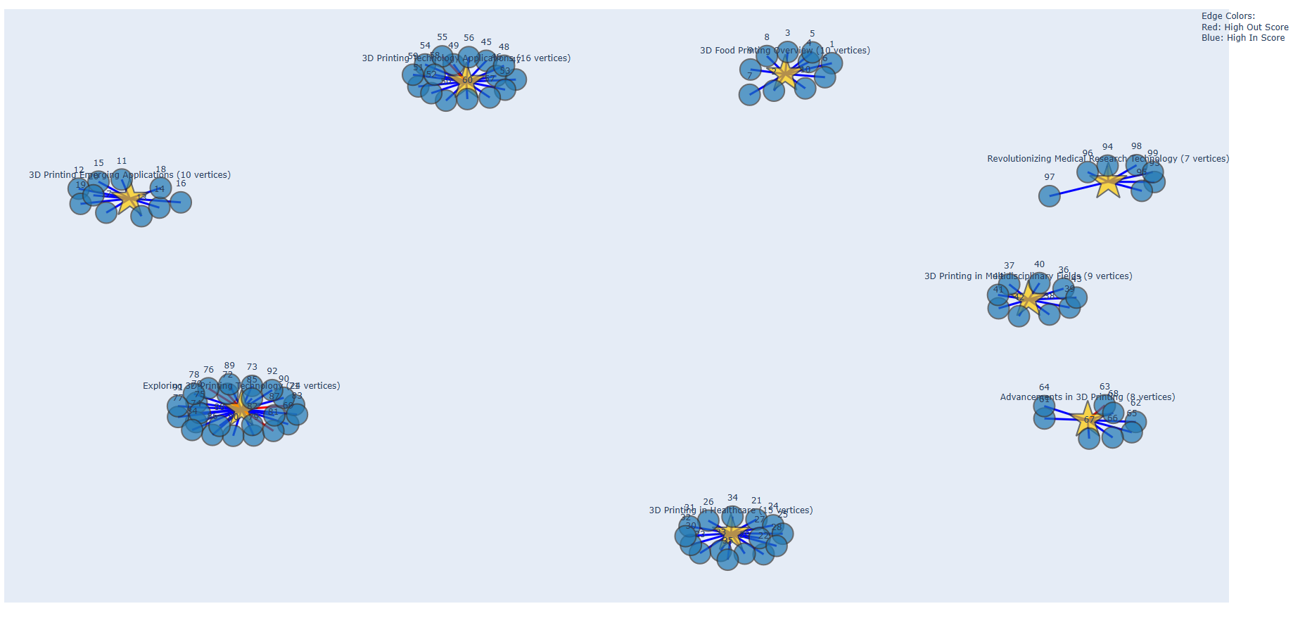
- The interactive HTML graph, which is saved at
Results/html/name.html
Release history Release notifications | RSS feed


Download files
Download the file for your platform. If you're not sure which to choose, learn more about installing packages.
Source Distribution
Built Distribution
Filter files by name, interpreter, ABI, and platform.
If you're not sure about the file name format, learn more about wheel file names.
Copy a direct link to the current filters
File details
Details for the file graphclusterer-0.2.3.tar.gz.
File metadata
- Download URL: graphclusterer-0.2.3.tar.gz
- Upload date:
- Size: 42.9 kB
- Tags: Source
- Uploaded using Trusted Publishing? No
- Uploaded via: twine/6.0.1 CPython/3.12.0
File hashes
| Algorithm | Hash digest | |
|---|---|---|
| SHA256 |
699d7f1c3d9ee22a33256d852f48a53c5dd8d716c481de38a7acff7ce135b1f1
|
|
| MD5 |
506c3f2e4bd5dd26cf598ba33254beec
|
|
| BLAKE2b-256 |
39f30de7dadadaabe62f3e9f129736f9152bd0a962624bd63dc869e6864db0b2
|
File details
Details for the file GraphClusterer-0.2.3-py3-none-any.whl.
File metadata
- Download URL: GraphClusterer-0.2.3-py3-none-any.whl
- Upload date:
- Size: 40.6 kB
- Tags: Python 3
- Uploaded using Trusted Publishing? No
- Uploaded via: twine/6.0.1 CPython/3.12.0
File hashes
| Algorithm | Hash digest | |
|---|---|---|
| SHA256 |
613250ad16b200e088af97c247962e7b99a8a303d641b6a2f2601155749318cf
|
|
| MD5 |
006afa27aca37ca0158fd524216a0523
|
|
| BLAKE2b-256 |
96f1703d094a902986bc45ca709365be15f015a8c9caef770c0094684129b17d
|


