

Badge |
Status |
|---|---|
Python versions |
|
Documentation |
|
Tests |
|
Coverage workflow |
|
PyPI package |
|
PyPI downloads |
|
Anaconda package |
|
Anaconda downloads |
|
Latest Anaconda release |









MomentRT
MomentRT is an open-source Python package for deterministic light transport using angular-moment methods. It models steady-state P1 diffusion in homogeneous infinite media and finite structured samples. Its API keeps the sample, illumination, mesh, and solver explicit, and its results include unit-bearing optical fields and power diagnostics.
Features
Analytical P1 diffusion from an isotropic point source in an infinite, homogeneous medium.
Boundary-aware P1 diffusion for finite samples, solved with linear tetrahedral finite elements.
Layered samples with box and sphere structures, plus resolved material cross-sections.
Explicit diffuse surface illumination and Robin or reflecting conditions on all six sample faces.
Interactive Plotly views for sample geometry, fluence, sections, and element-centered flux. Volume plots include an opacity control.
Unit-bearing fields, per-face escaping power, and solver diagnostics.
Circular contact detector apertures with explicit angular acceptance under a Lambertian escape model.
Tabulated wavelength-dependent materials and monochromatic sweeps on a fixed source, sample, and detector geometry.
Detector mesh-refinement studies and reusable finite-element preparation across wavelengths.
A coupled SP3 finite-element solver with explicit scattering anisotropy and matched-index boundaries, alongside the P1 diffusion solver.
A full three-dimensional P3 finite-element solver with matched-index faces.
Scalar Henyey–Greenstein, isotropic, Rayleigh, and tabulated scattering phase functions for SP3 and P3.
MomentRT offers P1, SP3, and P3 approximations. It does not currently solve the full radiative transfer equation or implement collimated LED propagation, free-space detector optics, broadband spectral integration, time dependence, or inverse estimation. Read the scientific guide for the equations, approximations, validation limits, and complete workflow.
Installation
Install the released Python package with Plotly visualization support:
python -m pip install "MomentRT[viz]"Or install the conda package and its dependencies:
conda install -c martinpdes -c conda-forge momentrtVerify the installation with the same Python interpreter you will use for your calculations:
python -c "import MomentRT; print(MomentRT.__version__)"The base package includes the numerical dependencies. Plotly is optional for interactive plots; PyVista is optional for VTK export. Install both plotting extras with python -m pip install "MomentRT[viz,vtk]".
First simulation
The infinite-medium solver is a quick way to calculate and inspect a fluence field. This example uses explicit units and places the source between grid nodes, avoiding the singular point-source location.
import numpy as np
import MomentRT

from MomentRT import (
    CartesianMesh,
    HomogeneousMedium,
    InfiniteDiffusion,
    Material,
    PointSource,
    Simulation,
    ureg,
)

material = Material(
    absorption=0.02 / ureg.millimeter,
    reduced_scattering=1.0 / ureg.millimeter,
    refractive_index=1.4,
    phase_function=MomentRT.phase_function.HenyeyGreenstein(),
)

medium = HomogeneousMedium(material=material)

mesh = CartesianMesh(
    shape=(40, 40, 40),
    spacing=np.full(3, 0.4) * ureg.millimeter,
    origin=np.full(3, -7.8) * ureg.millimeter,
)

source = PointSource(
    position=np.zeros(3) * ureg.millimeter,
    wavelength=970 * ureg.nanometer,
    optical_power=1 * ureg.milliwatt,
)

solver = InfiniteDiffusion()

simulation = Simulation(
    medium=medium,
    source=source,
    mesh=mesh,
    solver=solver,
)

result = simulation.run()

figure = result.fluence.plot(
    scale="log",
)
result.fluence is a nodal fluence-rate field with units of W/m². The infinite solver evaluates an analytical Green function; the observation grid does not create physical sample boundaries.
Finite-sample FEM workflow
For a finite sample, define its geometry and materials, create a mesh, specify surface illumination and all six boundary faces, then run Diffusion. This example uses the same explicit effective reflectance on each face and a circular diffuse source on the upper face.
import numpy as np
import MomentRT

from MomentRT import (
    CartesianMesh,
    Diffusion,
    Material,
    RobinBoundary,
    Simulation,
    StructuredMedium,
    SurfaceSource,
    ureg,
)

background = Material(
    absorption=0.02 / ureg.millimeter,
    reduced_scattering=1.0 / ureg.millimeter,
    refractive_index=1.4,
    phase_function=MomentRT.phase_function.HenyeyGreenstein(),
)

upper_material = Material(
    absorption=0.04 / ureg.millimeter,
    reduced_scattering=1.5 / ureg.millimeter,
    refractive_index=1.4,
    phase_function=MomentRT.phase_function.HenyeyGreenstein(),
)

sample = StructuredMedium(
    origin=(-4, -4, 0) * ureg.millimeter,
    size=(8, 8, 4) * ureg.millimeter,
)

sample.add_background(material=background)

sample.add_layer(
    name="Upper layer",
    thickness=1 * ureg.millimeter,
    material=upper_material,
)

mesh = CartesianMesh.from_sample(
    sample=sample,
    shape=(25, 25, 17),
)

source = SurfaceSource(
    face="z_min",
    position=np.array([0, 0, 0]) * ureg.millimeter,
    radius=1 * ureg.millimeter,
    wavelength=970 * ureg.nanometer,
    optical_power=1 * ureg.milliwatt,
)

boundary = RobinBoundary(effective_reflectance=0.5)

solver = Diffusion(
    boundaries={
        "x_min": boundary,
        "x_max": boundary,
        "y_min": boundary,
        "y_max": boundary,
        "z_min": boundary,
        "z_max": boundary,
    },
)

simulation = Simulation(
    medium=sample,
    source=source,
    mesh=mesh,
    solver=solver,
)

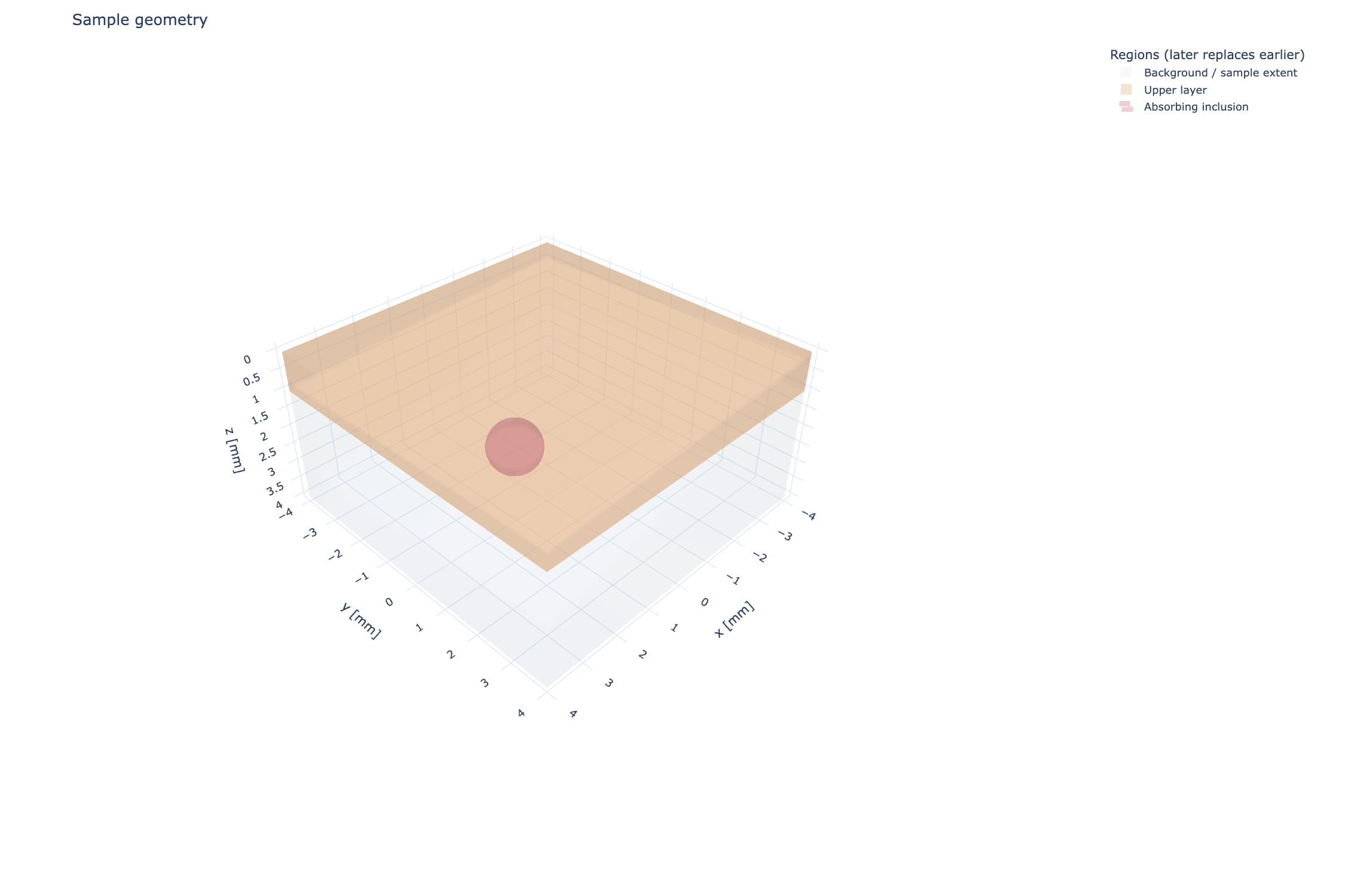
geometry = simulation.plot_system(
    show=False,
)

result = simulation.run()

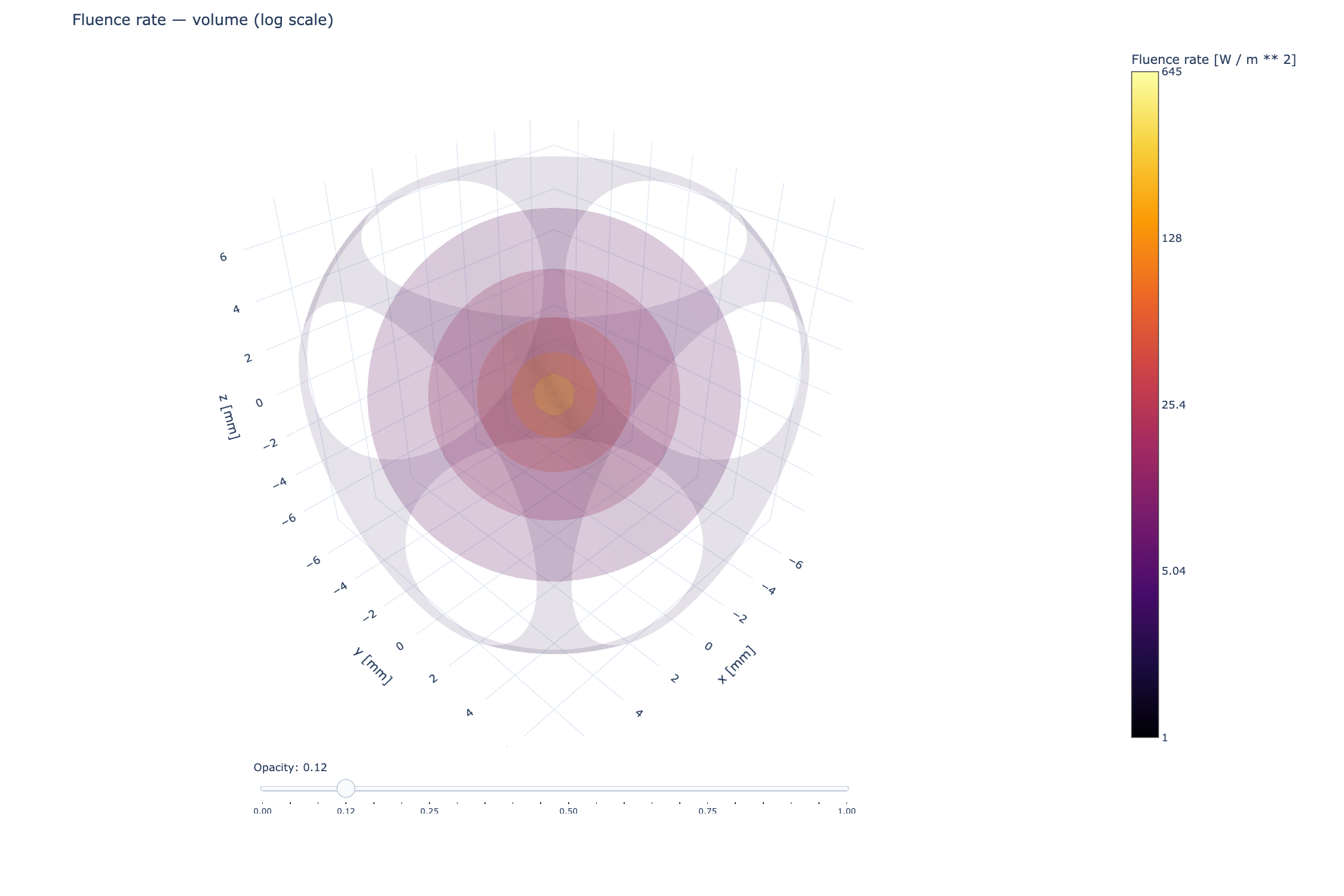
figure = result.fluence.plot(
    view="volume",
    scale="log",
)

print(f"Incoming power: {result.energy_balance['incoming_power']}")
print(f"Absorbed power: {result.energy_balance['absorbed_power']}")
print(f"Escaping power: {result.energy_balance['escaping_power']}")
The finite Diffusion solver uses P1 diffusion with linear tetrahedral FEM. Its sample mesh must span the sample exactly. Internal refractive indices must be equal because the solver models continuous fluence and does not resolve refracting interfaces. SurfaceSource.optical_power is diffuse power already coupled into the sample; incident beam propagation and specular entry losses are not included. The supplied effective reflectance is a diffuse partial-current coefficient, not a Fresnel value inferred from refractive index.
Visualization
The default fluence plot is a Plotly volume view. Adjust opacity from 0 to 1 using its browser slider, or choose a starting value with opacity:
figure = result.fluence.plot(
    view="volume",
    scale="log",
    opacity=0.12,
    show=False,
)

figure.write_html("fluence.html")
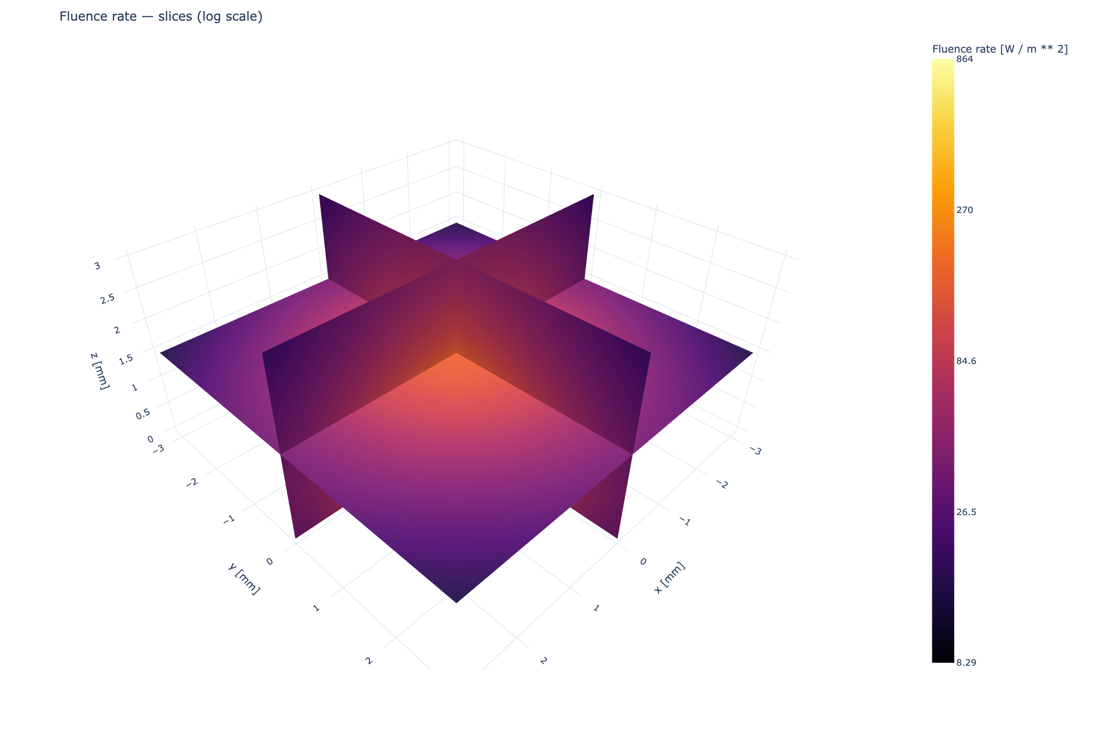
Other scalar-field views include central mesh slices and isosurfaces. result.flux.plot() displays element-centered diffusive flux vectors. sample.plot() shows the transparent construction surfaces; sample.plot_section(...) displays a sampled material or optical-property map. Log color scales change the displayed colors only; hover values retain their physical units.
The following figures were generated from MomentRT examples and results. The live documentation contains interactive Plotly versions.
Documentation
The online documentation includes:
The P1 moment equations, infinite-medium Green function, and approximation limits.
The finite-sample Robin boundary condition, weak form, and FEM assembly.
Complete workflows, visualization guidance, results, and API reference.
An executable example gallery.
Build the docs and run the examples locally with:
python -m pip install -e ".[documentation,viz]"
make docs PYTHON=.venv/bin/python
Common issues
Point-source singularity: do not place an observation node exactly at the point source. MomentRT reports this instead of silently regularizing it.
No visible internal interface: construction plots use transparent geometry surfaces. Use a sampled section to inspect the resolved material precedence.
Finite solver rejects refractive indices: the current FEM formulation requires equal internal refractive indices; it does not model internal refraction.
Unexpected surface-source power: source power is already coupled diffuse power in the sample. Collimated illumination and specular entry losses are outside the model.
Slow or changing fields under refinement: element-centroid materials, source quadrature, interface alignment, and P1 validity can all affect the result. Refine meshes and compare independent references; energy balance alone does not validate the physical approximation.
Log plot rejects values: logarithmic rendering requires strictly positive values and does not clip zeros or negative values.
Developer setup
Clone the repository, install the development extras, and build the docs with the same Python interpreter used for development:
git clone https://github.com/MartinPdeS/MomentRT.git
cd MomentRT
python3 -m venv .venv
.venv/bin/python -m pip install -e ".[testing,documentation,dev,viz]"
make check PYTHON=.venv/bin/python
make docs PYTHON=.venv/bin/python
make check runs quality checks and tests. The codebase intentionally keeps the package flat, with type hints and NumPy-style API docstrings. Run make typecheck docstring-check to validate annotations and public parameter documentation.
Citation and license
MomentRT is distributed under the MIT license. If you use it in research, cite the version recorded in CITATION.cff. For bibliographic metadata, see the CITATION.cff file.
1 maintainer

Metadata
1 maintainer
Release files for MomentRT 0.8.3
For a detailed explanation of source distributions (sdists) and built distributions (wheels), please see the package formats documentation.
Source distribution (sdist)
| File | Size | Uploaded | Provenance | Actions |
|---|---|---|---|---|
| momentrt-0.8.3.tar.gz | 80.5 kB | Without provenance | Details for momentrt-0.8.3.tar.gz |
Built distribution (wheel)
| File | Interpreter | ABI | Platform | Actions Reset |
|---|---|---|---|---|
| momentrt-0.8.3-py3-none-any.whl | Python 3 | none | any | Details for momentrt-0.8.3-py3-none-any.whl |
Total release size: 169.2 kB
Release files / momentrt-0.8.3.tar.gz
| Download URL | momentrt-0.8.3.tar.gz |
|---|---|
| Size | 80.5 kB |
| Tags | Source |
|
SHA-256 checksum How to use checksums |
dbafe29966b80d20edd443d2dd3767adeae30b957011b7b5d2ec8f7f8ddc8fb8
|
|
BLAKE2b-256 checksum How to use checksums |
bfc3aaa3c4acb56fc14a4fe36fae395ebc304df8ce848c3be10778589c37297b
|
| Upload date | |
|
Uploaded using Trusted Publishing? What is trusted publishing? |
No |
| Uploaded via |
twine/7.0.0 CPython/3.11.17
|
Release files / momentrt-0.8.3-py3-none-any.whl
| Download URL | momentrt-0.8.3-py3-none-any.whl |
|---|---|
| Size | 88.7 kB |
| Tags | Python 3 |
|
SHA-256 checksum How to use checksums |
a09c6aea2f60fb6d511b0fd7d2008566cff140ad6839378ded6b8cddfd183d2f
|
|
BLAKE2b-256 checksum How to use checksums |
5b8d97cfceb38cf108a2af6d398f787efd3f6681456d623e388381f5d568f2f7
|
| Upload date | |
|
Uploaded using Trusted Publishing? What is trusted publishing? |
No |
| Uploaded via |
twine/7.0.0 CPython/3.11.17
|
Security for MomentRT 0.8.3
Provenance
Provenance describes where a file came from. On PyPI, provenance is shared via attestations, which provide a verifiable record of the build or publishing details. View details, limitations and caveats.
No provenance found
None of the files in this release were uploaded with provenance metadata.
A note on package security
PyPI is a repository for distributing packages, not a service for auditing them. While third-party security researchers and our staff do their best to detect and remove malicious packages, PyPI cannot guarantee the quality, security or suitability of any given package.
To learn more about protecting yourself from malicious actors, visit our package security documentation.














