

OTSOpy





Python package version of the OTSO tool used for trajectory computations of charged particles in the Earth's magnetosphere.
OTSO is designed to be open-source; all suggestions for improvement are welcome, and please report any bugs you find. I welcome any help provided by the community in the development of OTSO.
Supported Python Versions: 3.11, 3.12, 3.13, and 3.14 (I will endeavour to keep OTSO support as up to date as possible)
OTSO Documentation
Detailed OTSO documentation for functions and input parameters is provided digitally via GitHub pages. Documentation can be found by clicking on OTSOdocs.
Installation
Installation of OTSOpy is designed to be as simple as possible and can be done utilising pip. Users have two options when downloading OTSOpy.
Option 1: PyPi
Users may install OTSO directly from PyPi using:
pip install OTSO
This will install OTSO into your current Python environment.
Option 2: Repository
Users may clone the repository and run the setup.py file within the main OTSOpy directory using:
pip install .
This will install OTSO into your current Python environment.
Troubleshooting
LINUX
Sometimes there are errors regarding libgfortran. Make a note of the libgfortran error message and then install the appropriate libgfortran version that is being requested. This should resolve the issue.
MAC
The compiled fortran libraries can be flagged as potential malware. To resolve this you can attempt to compile the libraries yourself or in your settings grant permission for your computer to access the required .so file.
Functions
Cutoff
Computes the geomagnetic cut-off rigidities for given locations around the Earth under user-inputted geomagnetic conditions.
Cone
Computes the asymptotic viewing directions for given locations around the Earth. Asymptotic latitudes and longitudes over a range of rigidity values are computed. Asymptotic latitude and longitude can be given in any available coordinate system.
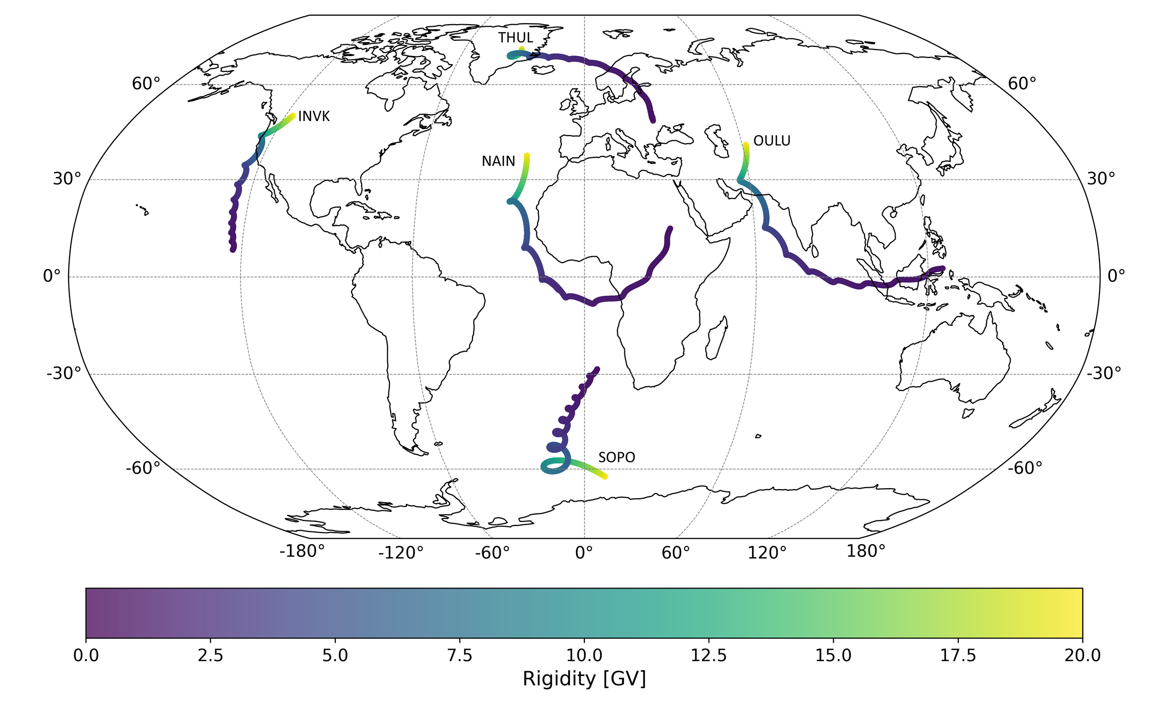
Figure 2: Asymptotic cones for the Oulu, Nain, South Pole, Thule, and Inuvik neutron monitors for the IGRF 2010 epoch and TSY89c model, with kp = 0. Latitudes and longitudes are in the geocentric coordinate system.
Trajectory
Computes and outputs the trajectory of a charged particle with a specified rigidity from a given start location on Earth. Positional information can be in any of the available coordinate systems.
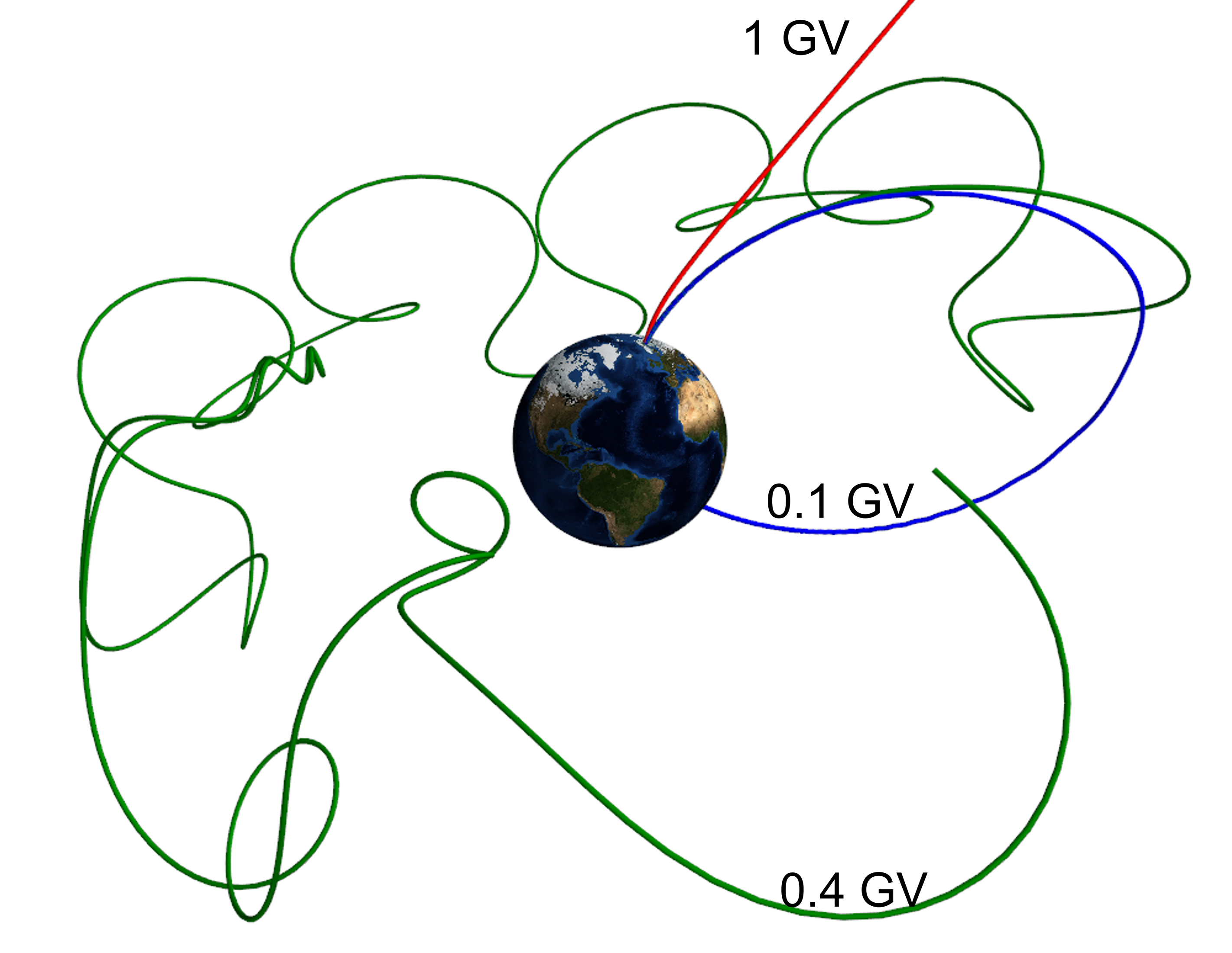
Figure 3: Computed trajectories of three cosmic rays of various rigidity values being backtraced from the Oulu neutron monitor for the IGRF 2000 and TSY89 model, with kp = 0. The 1GV particle is allowed (able to escape the magnetosphere); the 0.4GV particle is forbidden (it is trapped in the magnetosphere); and the 0.1GV is also forbidden (it returns to Earth).
Planet
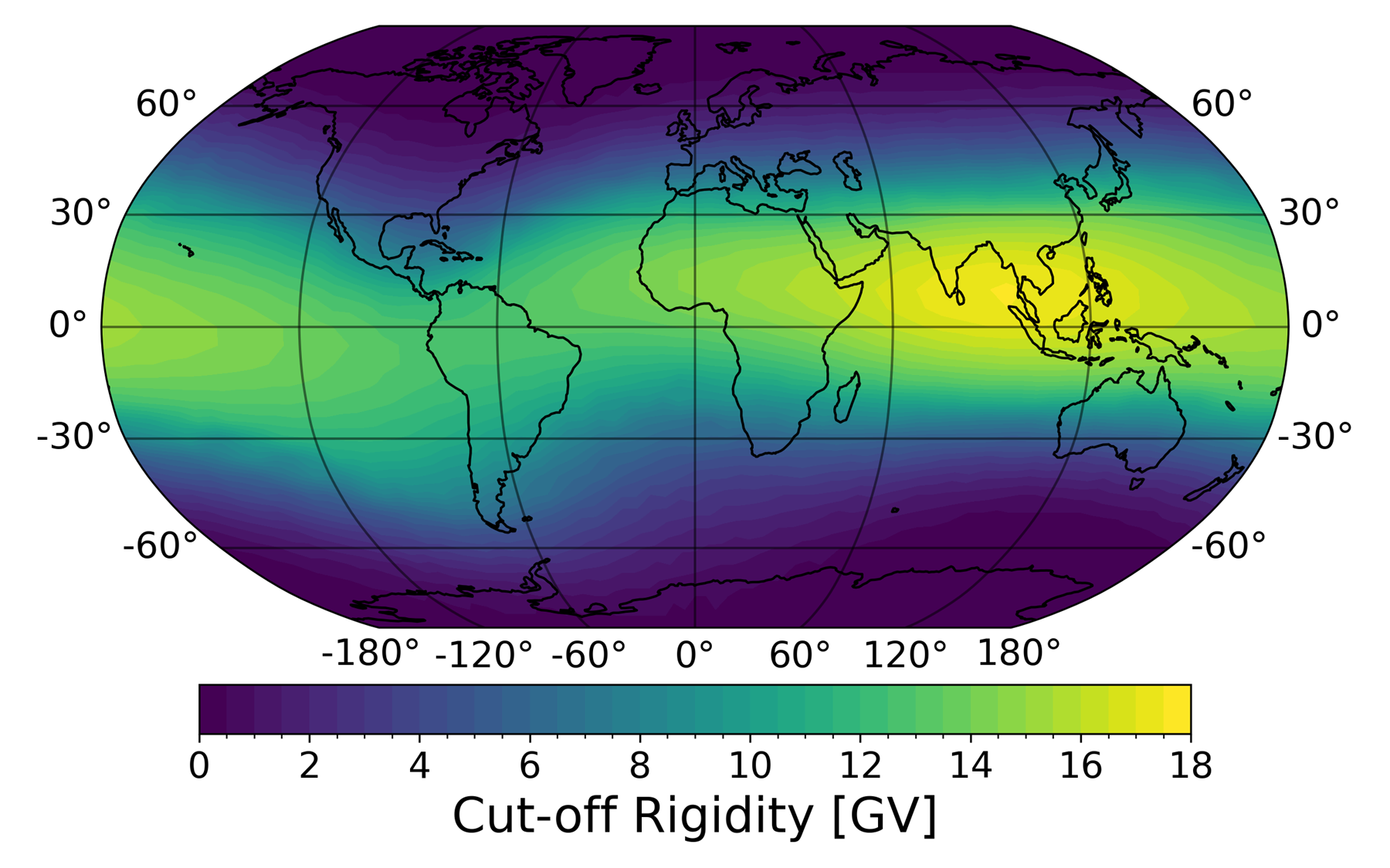
Performs the cutoff function over a user-defined location grid, allowing for cutoffs for the entire globe to be computed instead of individual locations. There is the option to return the asymptotic viewing directions at each computed location by utilising a user-inputted list of rigidity levels.
Flight
Computes the cut-off rigidities along a user-defined path. The function is named Flight as it is primarily been developed for use in aviation tools, but any path can be entered. For example, the function can be applied to geomagnetic latitude surveys using positional data from a ship voyage, or it can be used to compute anisotropy and cut-off values for low-Earth orbit spacecraft. This function allows for changing altitude, location, and date values.
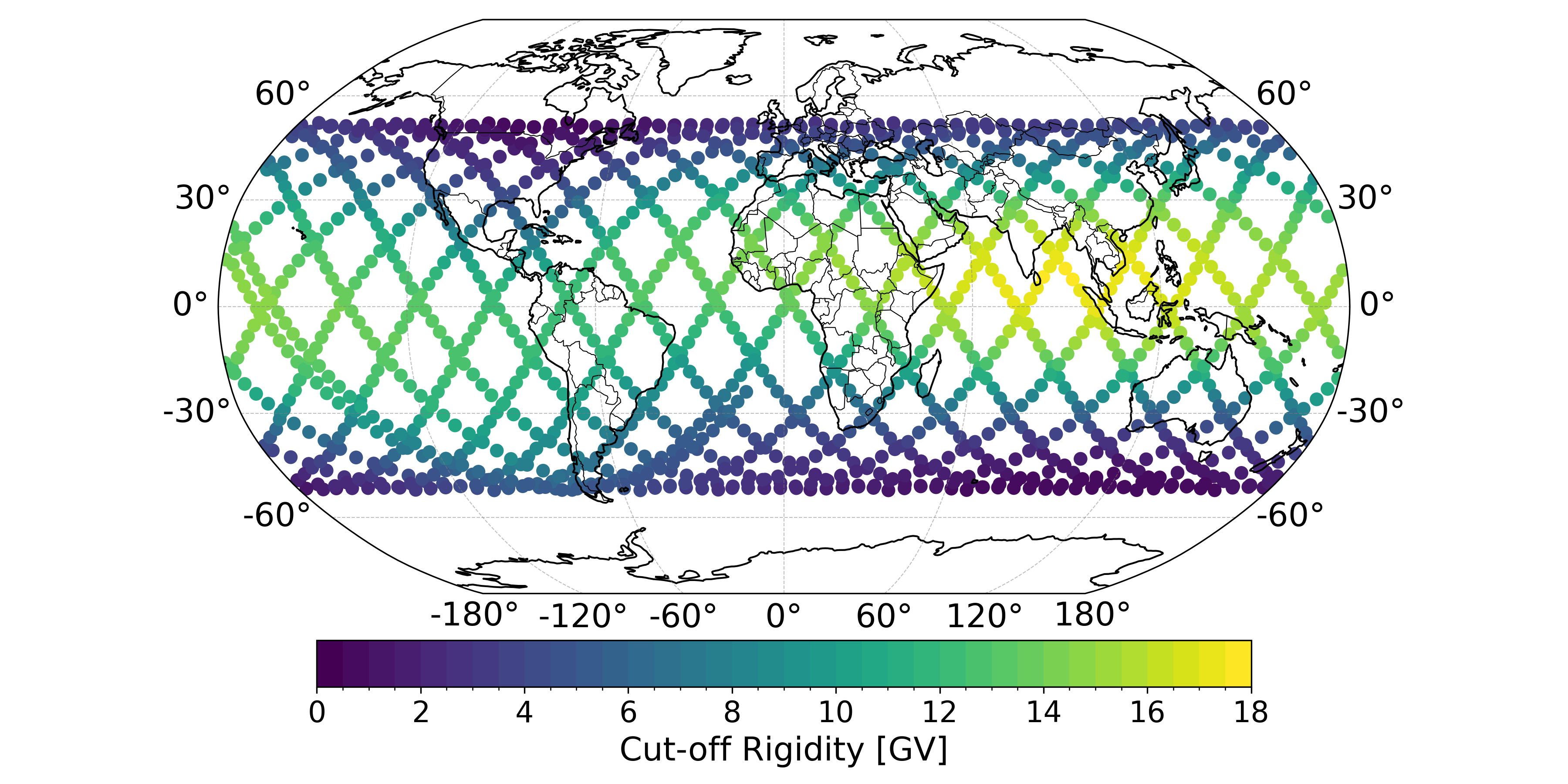
Figure 3: Computed effective vertical cut-off rigidities for the ISS between the 15th and 16th of March 2021. Geomagnetic parameters were extracted directly from OMNI for this period.
Skymap
Computes cutoff rigidities (Ru, Rc, Rl) over a grid of incoming zenith and azimuth angles for a given location, producing an angular map of cosmic ray access ("skymap") as seen from that point.
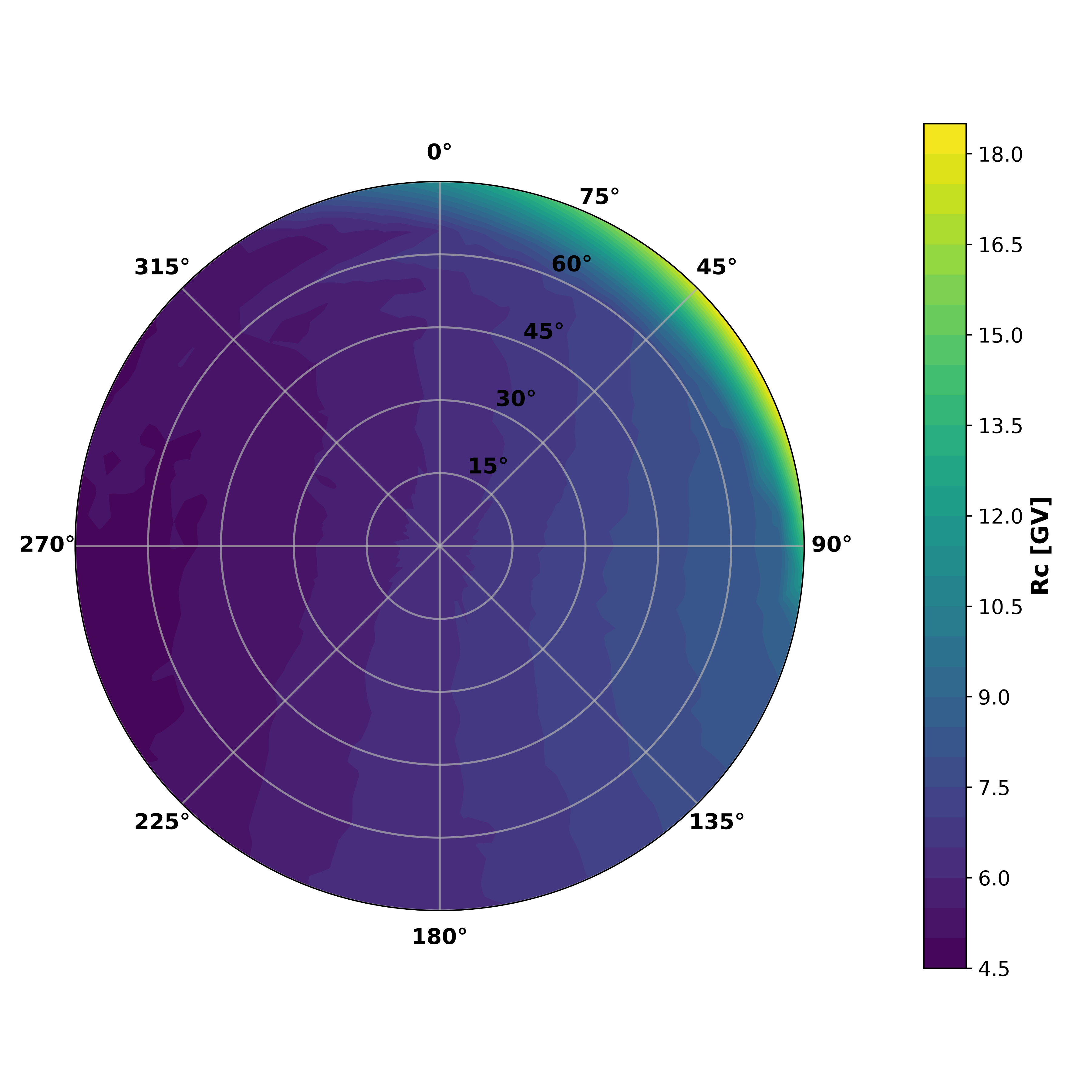
Figure 4: Cut-off skymap for the Rome NM. Cut-off values were computed in a 5°x5° zenith and azimuth grid between zenith 0°-75° and azimuth range 0°-365°.
Transmission
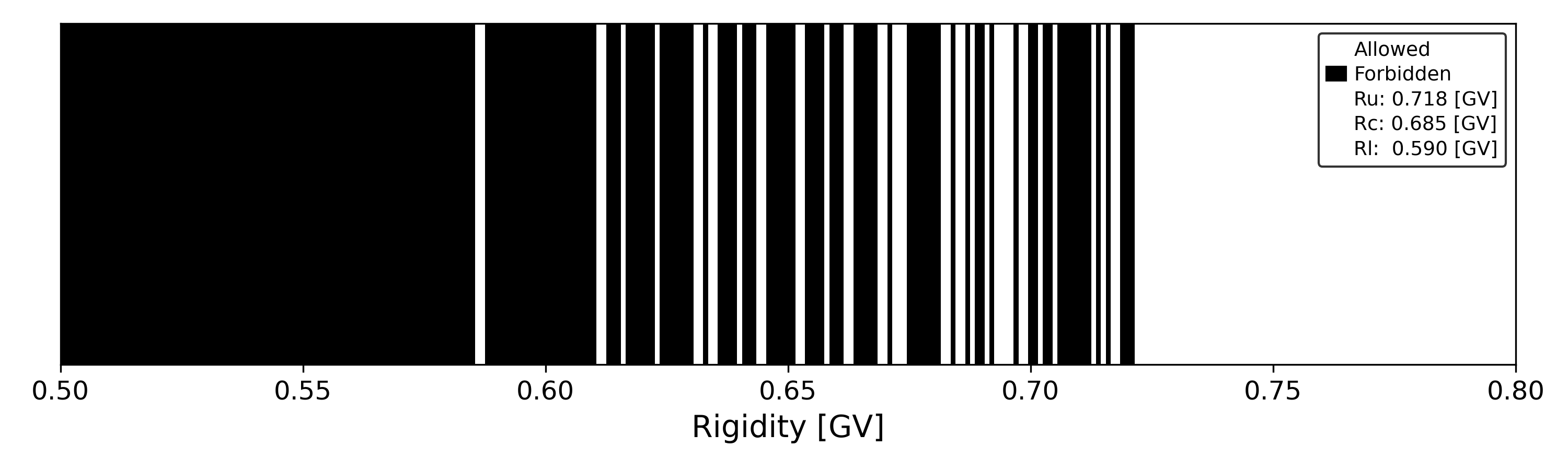
Computes the transmission function: the probability that a particle of a given rigidity has an allowed trajectory, obtained by sampling multiple trajectories per rigidity step. This gives a smoothed alternative to the sharp Ru/Rc/Rl cutoff values, particularly useful within the penumbra.
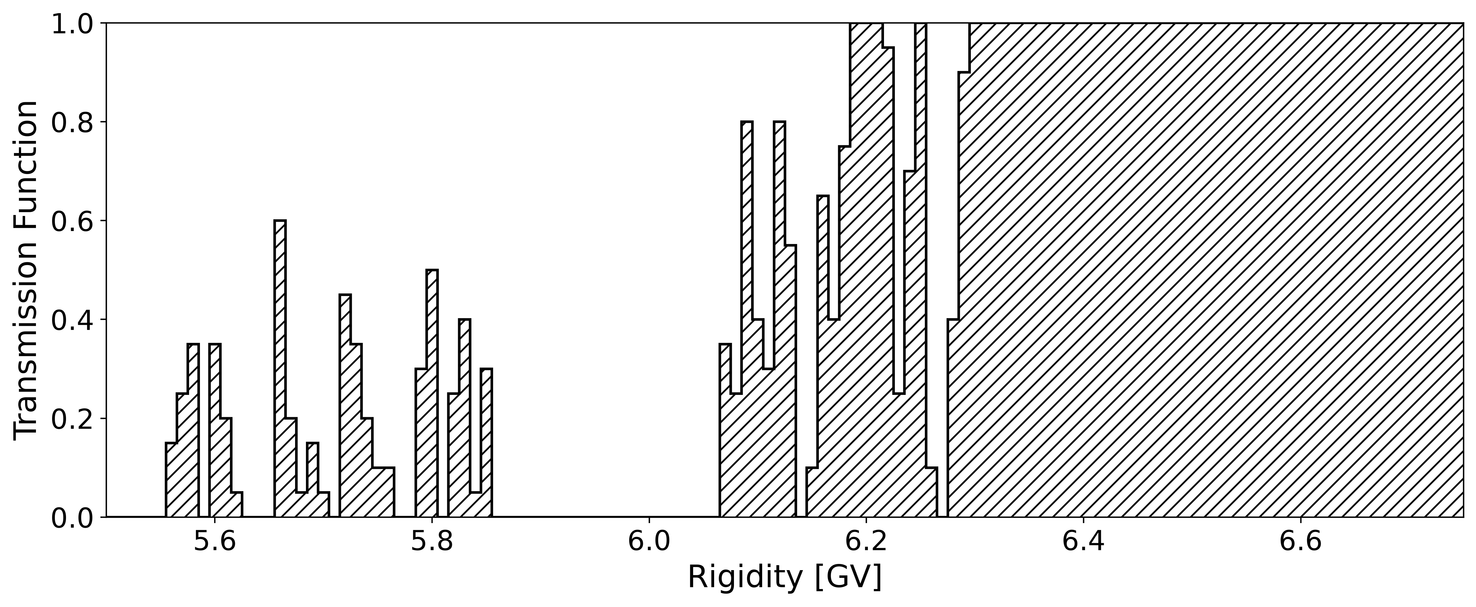
Figure 5: Computed transmission functions as a function of rigidity for the Rome NM. The penumbra region is highlighted as all rigidity values below and above those shown have 0 and 1, respectively.
Trace
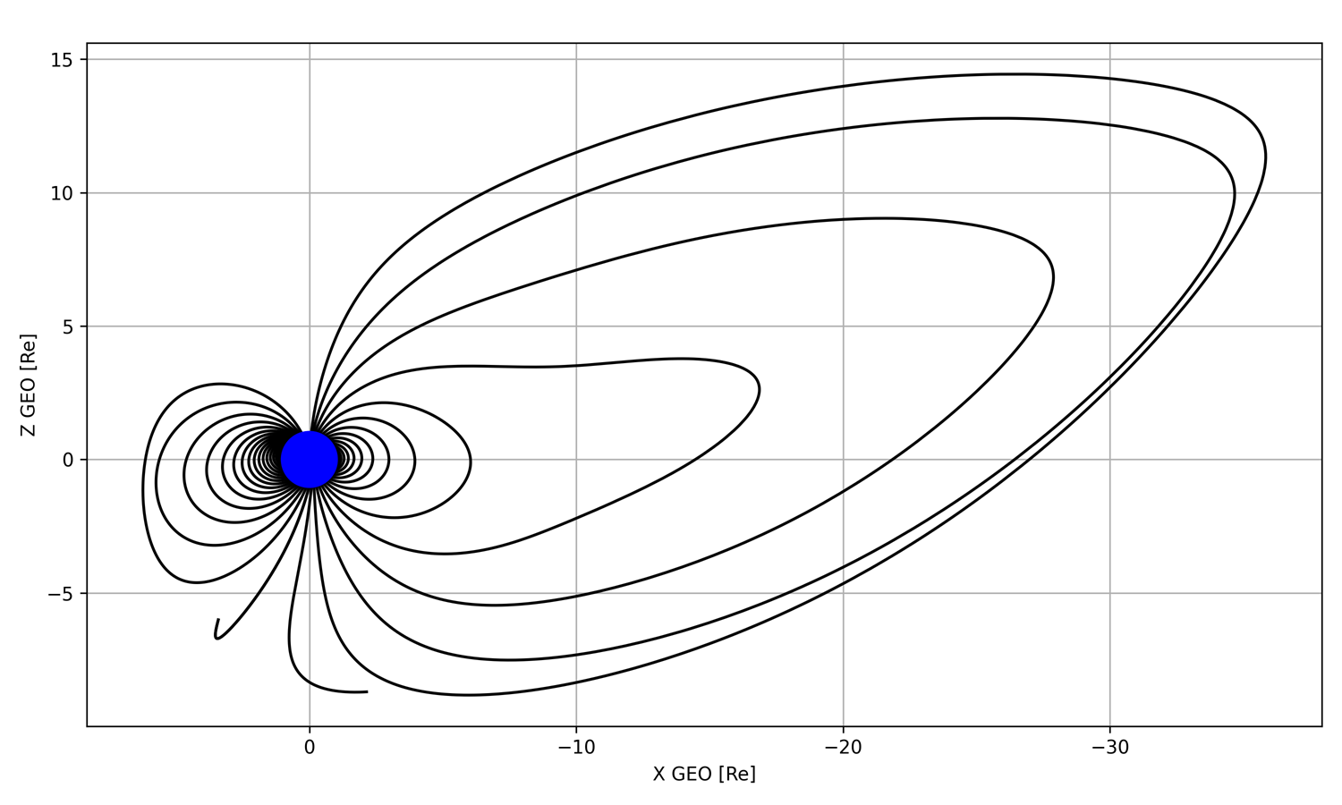
Traces the magnetic field lines around the globe or for a given location based on the geomagnetic configuration detailed by the user. It is useful for modelling the magnetosphere structure under disturbed conditions and for finding open magnetic field lines.
Coordtrans
Converts input positional information from one coordinate system to another, utilising the IRBEM library of coordinate transforms.
Magfield
Computes the total magnetic field strength at a given location depending on the user's input geomagnetic conditions. Outputs will be in the geocentric solar magnetospheric (GSM) coordinate system.
Examples
Cutoff
from OTSO import cutoff

if __name__ == '__main__':

    stations_list = ["OULU", "ROME", "ATHN", "CALG"]  # list of neutron monitor stations (using their abbreviations)

    cutoff_results = cutoff(
        Stations=stations_list,
        computation_params={"corenum": 1, "threadnum": 4},
        datetime_params={"year": 2000, "month": 1, "day": 1, "hour": 0}
    )

    print(cutoff_results[0])  # dataframe output containing Ru, Rc, Rl for all input locations
    #print(cutoff_results[1]) # dataframe output containing asymptotic viewing direction results for all input locations
    #print(cutoff_results[2]) # dataframe output containing transmission functions for all input locations
    print(cutoff_results[-1]) # text output of input variable information
Output
Ru = upper cut-off rigidity [GV]
Rc = effective cut-off rigidity [GV]
Rl = lower cut-off rigidity [GV]
PTF = Penumbral Transmission Function
     ATHN  CALG  OULU  ROME
Ru   9.15  1.12  0.72  6.40
Rc   8.79  1.08  0.68  6.27
Rl   7.56  1.00  0.60  5.69
PTF  0.23  0.33  0.33  0.18
Cone
from OTSO import cone

if __name__ == '__main__':

    stations_list = ["OULU", "ROME", "ATHN", "CALG"]  # list of neutron monitor stations (using their abbreviations)

    cone_results = cone(
        Stations=stations_list,
        computation_params={"corenum": 1, "threadnum": 4},
        datetime_params={"year": 2000, "month": 1, "day": 1, "hour": 0},
        coordinate_params={"coodsystem": "GEO"}
    )

    print(cone_results[0])  # dataframe output containing asymptotic cones for all input locations
    #print(cone_results[1])  # dataframe output containing Ru, Rc, Rl for all inputted locations
    print(cone_results[-1])  # text output of input variable information
Output
Showing only the cone[0] output containing the asymptotic viewing directions of the input stations. Result layout is: filter;latitude;longitude. Asymptotic latitude and longitude will be in the coordinate system assigned by the user with the "coordsystem" option. If the filter value is 1, then the particle of that rigidity has an allowed trajectory. If the filter value is NOT 1, then the particle of that rigidity has a forbidden trajectory.
      R [GV]                 ATHN                 CALG                OULU                 ROME
0       0.01    -1;2.0108;44.0606  -1;35.8351;209.8197  -1;70.0382;65.1090   -1;49.2027;16.2981
1       0.02  -1;-13.0490;20.5069   -1;6.1502;221.3774  -1;64.4879;66.7135   -1;15.8190;32.2432
2       0.03   -1;-11.7351;9.6165  -1;11.7782;205.3306  -1;62.0193;66.2900  -1;30.5232;340.8636
3       0.04   -1;42.3357;30.1360  -1;25.1684;235.4000  -1;60.4429;65.9669    -1;1.2832;12.0507
4       0.05  -1;25.9424;349.9241  -1;37.4414;214.7077  -1;72.7436;65.6391   -1;18.9000;33.8198
...      ...                  ...                  ...                 ...                  ...
1995   19.96  1;-13.9059;270.7747   1;29.5393;100.1982  1;18.5610;231.5551  1;-15.1452;250.7234
1996   19.97  1;-13.8933;270.7377   1;29.5522;100.2077  1;18.5730;231.5530  1;-15.1270;250.6970
1997   19.98  1;-13.8807;270.7007   1;29.5647;100.2165  1;18.5850;231.5509  1;-15.1088;250.6706
1998   19.99  1;-13.8681;270.6638   1;29.5773;100.2253  1;18.5970;231.5488  1;-15.0906;250.6443
1999   20.00  1;-13.8555;270.6269   1;29.5901;100.2348  1;18.6090;231.5467  1;-15.0724;250.6180
Trajectory
from OTSO import trajectory

if __name__ == '__main__':

    stations_list = ["OULU", "ROME", "ATHN", "CALG"]  # list of neutron monitor stations (using their abbreviations)

    trajectory_results = trajectory(
        Stations=stations_list,
        particle_params={"rigidity": 5},
        computation_params={"corenum": 1}
    )

    print(trajectory_results[0])  # dictionary output containing positional information for all trajectories generated starting
                                   # from input stations
    print(trajectory_results[-1])  # text output of input variable information
Output
Showing the dataframe produced for the particle originating from Oulu. Other trajectories are within the trajectory[0] dictionary. Additionally the Filter value, letting you know if the trajectory is allowed or not, and the asymptotic latitude and longitude at the end point is included.
{'station': 'OULU', 'rigidity': 5, 'Filter': 1, 'Alat': 17.686, 'Along': 71.645,
'trajectory':
        GSM_X [Re]  GSM_Y [Re]  GSM_Z [Re]  GSM_Vx [km/s]  GSM_Vy [km/s]  GSM_Vz [km/s]
0       0.000758    0.337510    0.945797    -363.627474  102565.136125  276221.900492
1       0.000751    0.338497    0.948354    -752.912094  106092.859038  274885.459909
2       0.000742    0.339516    0.950899    -947.661814  109593.008563  273508.230399
3       0.000733    0.340568    0.953430    -952.202373  113055.913496  272095.077903
4       0.000726    0.341651    0.955948    -771.327333  116472.447095  270650.793101
...          ...         ...         ...            ...            ...            ...
4342    4.339465   10.034078    5.789009   88563.413393  266373.057077   89555.535598
4343    4.340289   10.036556    5.789842   88556.841197  266375.796135   89553.887663
4344    4.341112   10.039035    5.790675   88550.270023  266378.534116   89552.241321
4345    4.341936   10.041513    5.791508   88543.699871  266381.271023   89550.596572
4346    4.342760   10.043991    5.792341   88537.130739  266384.006855   89548.953413

[4347 rows x 6 columns]}
Planet
from OTSO import planet

if __name__ == '__main__':

    # cutoff_comp can be set as "Vertical, Apparent, and Custom"
    planet_results = planet(
        cutoff_comp="Vertical",
        computation_params={"corenum": 1, "threadnum": 4},
        datetime_params={"year": 2000},
        rigidity_params={"rigiditystep": 0.1}
    )

    print(planet_results[0]) # dataframe containing cutoff results for planet grid
    #print(planet_results[1]) # dataframe output containing asymptotic viewing directions for planet grid
    #print(planet_results[2]) # dataframe output containing transmission functions for the planet grid
    print(planet_results[-1]) # text output of input variable information
Output
The default output is a 5°x5° grid of the Earth with no asymptotic viewing directions or transmission functions computed.
      Latitude  Longitude  Ru [GV]  Rc [GV]  Rl [GV]  PTF
0        -90.0        0.0      0.0      0.0      0.0  0.0
1        -90.0        5.0      0.0      0.0      0.0  0.0
2        -90.0       10.0      0.0      0.0      0.0  0.0
3        -90.0       15.0      0.0      0.0      0.0  0.0
4        -90.0       20.0      0.0      0.0      0.0  0.0
...        ...        ...      ...      ...      ...  ...
2696      90.0      340.0      0.0      0.0      0.0  0.0
2697      90.0      345.0      0.0      0.0      0.0  0.0
2698      90.0      350.0      0.0      0.0      0.0  0.0
2699      90.0      355.0      0.0      0.0      0.0  0.0
2700      90.0      360.0      0.0      0.0      0.0  0.0
Flight
from OTSO import flight
import datetime

if __name__ == '__main__':

    latitude_list = [10, 15, 20, 25, 30]  # [Latitudes]
    longitude_list = [10, 15, 20, 25, 30]  # [Longitudes]
    altitude_list = [30, 40, 50, 60, 80]  # [Altitudes] in km
    date_list = [datetime.datetime(2000, 10, 12, 8), datetime.datetime(2000, 10, 12, 9), datetime.datetime(2000, 10, 12, 10),
                 datetime.datetime(2000, 10, 12, 11), datetime.datetime(2000, 10, 12, 12)]  # [dates]

    flight_results = flight(
        latitudes=latitude_list,
        longitudes=longitude_list,
        dates=date_list,
        altitudes=altitude_list,
        cutoff_comp="Vertical",
        computation_params={"corenum": 1, "threadnum": 4},
    )

    print(flight_results[0]) # dataframe output containing Ru, Rc, Rl along flightpath
    print(flight_results[1]) # dataframe output containing asymptotic viewing directions
    print(flight_results[2])  # dataframe output containing transmission functions
    print(flight_results[-2]) # text output of input variable information
    print(flight_results[-1])  # dataframe output of input variables
Output
flight[0] dataframe output.
                  Date Latitude Longitude Altitude [km]  Ru [GV]  Rc [GV]  Rl [GV]   PTF
0  2000-10-12 08:00:00       10        10            30    16.18    16.18    16.18  0.00
1  2000-10-12 09:00:00       15        15            40    16.23    16.23    16.23  0.00
2  2000-10-12 10:00:00       20        20            50    15.66    15.66    15.66  0.00
3  2000-10-12 11:00:00       25        25            60    14.53    14.53    14.53  0.00
4  2000-10-12 12:00:00       30        30            80    12.85    12.25    11.04  0.33
Skymap
from OTSO import skymap

if __name__ == '__main__':

    stations_list = ["OULU"]  # list of neutron monitor stations (using their abbreviations)

    skymap_results = skymap(
        Stations=stations_list,
        computation_params={"corenum": 1, "threadnum": 4},
        datetime_params={"year": 2000, "month": 1, "day": 1, "hour": 0},
        rigidity_params={"startrigidity": 5, "endrigidity": 0, "rigiditystep": 0.01},
        skymap_params={"zenithstep": 30, "azimuthstep": 45, "maxzenith": 60}
    )

    print(skymap_results[0])  # dictionary of dataframes containing skymap results for each input location
    print(skymap_results[-1])  # text output of input variable information
Output
skymap_results[0] output showing the cutoff rigidities and penumbra transmission fraction (PTF) at each sampled zenith/azimuth angle for Oulu.
{'OULU':
    Zenith  Azimuth  Ru [GV]  Rc [GV]  Rl [GV]   PTF
0      0.0      0.0     0.72     0.68     0.58  0.29
1     30.0      0.0     0.74     0.72     0.65  0.22
2     30.0     45.0     0.74     0.70     0.60  0.29
3     30.0     90.0     0.73     0.72     0.65  0.12
4     30.0    135.0     0.75     0.73     0.60  0.13
5     30.0    180.0     0.72     0.68     0.61  0.36
6     30.0    225.0     0.71     0.68     0.63  0.38
7     30.0    270.0     0.69     0.66     0.64  0.60
8     30.0    315.0     0.71     0.70     0.64  0.14
9     30.0    360.0     0.74     0.72     0.65  0.22
10    60.0      0.0     0.72     0.67     0.61  0.45
11    60.0     45.0     0.75     0.69     0.61  0.43
12    60.0     90.0     0.75     0.69     0.65  0.60
13    60.0    135.0     0.74     0.71     0.63  0.27
14    60.0    180.0     0.72     0.69     0.63  0.33
15    60.0    225.0     0.68     0.67     0.65  0.33
16    60.0    270.0     0.70     0.66     0.59  0.36
17    60.0    315.0     0.71     0.64     0.60  0.64
18    60.0    360.0     0.72     0.67     0.61  0.45}
Transmission
from OTSO import transmission

if __name__ == '__main__':

    stations_list = ["OULU"]  # list of neutron monitor stations (using their abbreviations)

    transmission_results = transmission(
        Stations=stations_list,
        computation_params={"corenum": 1, "threadnum": 4},
        datetime_params={"year": 2000, "month": 1, "day": 1, "hour": 0},
        rigidity_params={"startrigidity": 0.8, "endrigidity": 0.5, "rigiditystep": 0.01},
        transmission_params={"transmissionsamples": 20}
    )


    print(transmission_results[0])  # dataframe output containing the transmission function for all input locations
    print(transmission_results[-1])  # text output of input variable information
Output
transmission_results[0] output showing the transmission fraction (TF) for Oulu across the penumbra, from fully forbidden (0.0) to fully allowed (1.0).
    R [GV]  OULU_TF
0     0.51     0.00
1     0.52     0.00
2     0.53     0.00
3     0.54     0.00
4     0.55     0.00
5     0.56     0.00
6     0.57     0.00
7     0.58     0.05
8     0.59     0.10
9     0.60     0.25
10    0.61     0.20
11    0.62     0.30
12    0.63     0.35
13    0.64     0.60
14    0.65     0.40
15    0.66     0.55
16    0.67     0.25
17    0.68     0.20
18    0.69     0.60
19    0.70     0.20
20    0.71     0.00
21    0.72     0.00
22    0.73     1.00
23    0.74     1.00
24    0.75     1.00
25    0.76     1.00
26    0.77     1.00
27    0.78     1.00
28    0.79     1.00
29    0.80     1.00
Trace
from OTSO import trace

if __name__ == '__main__':

    trace_results = trace(
        computation_params={"corenum": 1},
        grid_params={"latstep": -10, "longstep": 30}
    )

    print(trace_results[0]) # dictionary output containing positional information magnetic field lines generated over
                    # the globe
    print(trace_results[1]) # dataframe output containing L-shell and invariant latitude for each traced location
    print(trace_results[-1]) # text output of input variable information
Output
Example output of one of the field line traces for the location latitude = 60° and longitude = 215°. The L shell and Invariant Latitude are also computed from the magnetic field line tracing and provided in a seperate dataframe.
'20_30': {'altitude [km]': 20, 'Trace':
       X_GEO [Re]  Y_GEO [Re]  Z_GEO [Re]  Bx_GSM [nT]  By_GSM [nT]  Bz_GSM [nT]
0      0.529668    0.704775   -0.472005      26957.1      18082.7      9155.37
1      0.531030    0.705554   -0.471979      26830.5      18010.9      9208.75
2      0.532392    0.706332   -0.471948      26704.5      17939.1      9261.65
3      0.533755    0.707110   -0.471913      26579.0      17867.5      9314.08
4      0.535119    0.707887   -0.471874      26454.2      17796.0      9366.04
..          ...         ...         ...          ...          ...          ...
839    0.820910    0.475026    0.339936     -35322.8     -28268.5      4267.08
840    0.819794    0.474022    0.340397     -35491.9     -28402.6      4169.30
841    0.818677    0.473019    0.340854     -35661.9     -28537.4      4070.62
842    0.815315    0.470013    0.342207     -36176.3     -28945.5      3768.88
843    0.814191    0.469012    0.342652     -36349.3     -29082.8      3666.42

[844 rows x 6 columns]}
Coordtrans
from OTSO import coordtrans
import datetime

if __name__ == '__main__':

    lat_lon_alt_list = [[10, 10, 10]]  # [[Latitude,Longitude,Altitude]]
    date_list = [datetime.datetime(2000, 10, 12, 8)]  # [dates]

    # coordtrans uses individual parameters, not grouped ones
    Coords = coordtrans(
        Locations=lat_lon_alt_list,
        dates=date_list,
        CoordIN="GEO",
        CoordOUT="GSM",
        corenum=1
    )

    print(Coords[0])  # dataframe output of converted coordinates
    print(Coords[-1])  # text output detailing the initial and final conversion coordinate system
Output
Coords[0] output converting the [10,10,10] position from GEO coordinate system to GSM coordinate system.
                  Date X_GEO [Re] Y_GEO [Re] Z_GEO [Re] X_GSM [Re] Y_GSM [Re] Z_GSM [Re]
0  2000-10-12 08:00:00         10         10         10   12.41742  -1.097125   12.02514
Magfield
from OTSO import magfield

if __name__ == '__main__':

    location_list = [[10, 10, 10]]  # [[X,Y,Z]] Earth radii Geocentric coordinates in this instance

    magfield_results = magfield(
        Locations=location_list,
        coordinate_params={"inputcoord": "GDZ", "coordout": "GSM"},
        computation_params={"corenum": 1}
    )

    print(magfield_results[0])  # dataframe of returned magnetic field vectors at inputted locations
    print(magfield_results[-1])  # text output of input variable information
Output
magfield[0] output showing the magnetic field vector at the input location in the GSM coordinate system.
   altitude_GDZ [km]  latitude_GDZ  longitude_GDZ   GSM_Bx [nT]  GSM_By [nT]   GSM_Bz [nT]
0               10.0          10.0           10.0 -16685.751694  4567.896568  29247.384684
Acknowledgements
The fantastic IRBEM library has been used in the development of OTSO, which proved an invaluable asset and greatly sped up development. The latest release of the IRBEM library can be found at https://doi.org/10.5281/zenodo.6867552. Thank you to N. Tsyganenko for the development of the external magnetic field models and their code, which are used within OTSO.
Thank you to Don and Peggy Smart for their insightful discussion on the nature of cutoff computations and for providing me with a copy of their cutoff computation tool, from which I learned a lot and adopted many of their inspired optimisation techniques.
A wider thanks goes to the space physics community who, through the use of the original OTSO, provided invaluable feedback, advice on improvements, and bug reporting. All discussions and advice have aided in the continual development and improvement of OTSO, allowing it to fulfil its aim of being a community-driven open-source tool. The lessons learned from the initial OTSO versions have been incorporated into OTSOpy. Dr. Chris Davis was also instrumental in the development of OTSOpy with his suggestion of incorporating OTSO into the AniMARIE tool, initiating the package development and providing help by expanding functionality and bug fixing. OTSO was developed at the University of Oulu as part of the Academy of Finland QUASARE project. I would like to thank my colleagues at the University and the Academy of Finland for supporting the work.
OTSO in Publications
If you have used OTSO in your scientific research, please acknowledge it in your publication using the following sentence, or something similar.
"We acknowledge the use of the OTSO tool [VERSION USED], the latest version of which can be found at https://doi.org/10.5281/zenodo.15341361."
Additionally, due to the flexibility of OTSO and freedom of user input, it is recommended that, along with your publication, you attach a document detailing the specific inputs for your OTSO computations for reproducibility.
References
- Larsen, N., Mishev, A., & Usoskin, I. (2023). A new open-source geomagnetosphere propagation tool (OTSO) and its applications. Journal of Geophysical Research: Space Physics, 128, e2022JA031061. https://doi.org/10.1029/2022JA031061
1 maintainer

Download files
Download the file for your platform. If you're not sure which to choose, learn more about installing packages.
Source Distribution
Built Distribution
Filter files by name, interpreter, ABI, and platform.
If you're not sure about the file name format, learn more about wheel file names.
Copy a direct link to the current filters
File details
Details for the file otso-1.3.0.tar.gz.
File metadata
- Download URL: otso-1.3.0.tar.gz
- Upload date:
- Size: 13.6 MB
- Tags: Source
- Uploaded using Trusted Publishing? No
- Uploaded via:
twine/7.0.0 CPython/3.12.14
File hashes
| Algorithm | Hash digest | |
|---|---|---|
| SHA256 |
635b3327b9c5ba8ce3c77af3df11d6ff068800ec77f0e1adc445214d7a65469d
|
|
| MD5 |
06e80c7653b6ee88abd34fb0fc787ec7
|
|
| BLAKE2b-256 |
6e49b2e731a114c298ca61ff73e1a1c879028310922bcf809ed6fb3c60df691b
|
File details
Details for the file otso-1.3.0-py3-none-any.whl.
File metadata
- Download URL: otso-1.3.0-py3-none-any.whl
- Upload date:
- Size: 13.8 MB
- Tags: Python 3
- Uploaded using Trusted Publishing? No
- Uploaded via:
twine/7.0.0 CPython/3.12.14
File hashes
| Algorithm | Hash digest | |
|---|---|---|
| SHA256 |
4f7550aeab3ad96c57a31585e21fa7462f9521842ddf87e4e38ab197f3472725
|
|
| MD5 |
53af42d9e6fe628fe203b5cb911ab7a0
|
|
| BLAKE2b-256 |
060665d603b3c9297f8d65c57ff19d620e2ccf72a340ed4485d82fec90055740
|














