PyDTMC

PyDTMC is a full-featured and lightweight library for discrete-time Markov chains analysis. It provides classes and functions for creating, manipulating, simulating and visualizing Markov processes.

Status:
Info:
PyPI:
Conda:
Donation:

Requirements

The Python environment must include the following packages:

Notes:

It's recommended to install Graphviz and pydot before using the plot_graph function.
The packages pytest and pytest-benchmark are required for performing unit tests.
The package Sphinx is required for building the package documentation.

Installation & Upgrade

PyPI:

$ pip install PyDTMC
$ pip install --upgrade PyDTMC

Git:

$ pip install https://github.com/TommasoBelluzzo/PyDTMC/tarball/master
$ pip install --upgrade https://github.com/TommasoBelluzzo/PyDTMC/tarball/master

$ pip install git+https://github.com/TommasoBelluzzo/PyDTMC.git#egg=PyDTMC
$ pip install --upgrade git+https://github.com/TommasoBelluzzo/PyDTMC.git#egg=PyDTMC

Conda:

$ conda install -c conda-forge pydtmc
$ conda update -c conda-forge pydtmc

$ conda install -c tommasobelluzzo pydtmc
$ conda update -c tommasobelluzzo pydtmc

Usage: MarkovChain Class

The MarkovChain class can be instantiated as follows:

>>> p = [[0.2, 0.7, 0.0, 0.1], [0.0, 0.6, 0.3, 0.1], [0.0, 0.0, 1.0, 0.0], [0.5, 0.0, 0.5, 0.0]]
>>> mc = MarkovChain(p, ['A', 'B', 'C', 'D'])
>>> print(mc)

DISCRETE-TIME MARKOV CHAIN
 SIZE:           4
 RANK:           4
 CLASSES:        2
  > RECURRENT:   1
  > TRANSIENT:   1
 ERGODIC:        NO
  > APERIODIC:   YES
  > IRREDUCIBLE: NO
 ABSORBING:      YES
 MONOTONE:       NO
 REGULAR:        NO
 REVERSIBLE:     YES
 SYMMETRIC:      NO

Below a few examples of MarkovChain properties:

>>> print(mc.is_ergodic)
False

>>> print(mc.recurrent_states)
['C']

>>> print(mc.transient_states)
['A', 'B', 'D']

>>> print(mc.steady_states)
[array([0.0, 0.0, 1.0, 0.0])]

>>> print(mc.is_absorbing)
True

>>> print(mc.fundamental_matrix)
[[1.50943396, 2.64150943, 0.41509434]
 [0.18867925, 2.83018868, 0.30188679]
 [0.75471698, 1.32075472, 1.20754717]]
 
>>> print(mc.kemeny_constant)
5.547169811320755

>>> print(mc.entropy_rate)
0.0

Below a few examples of MarkovChain methods:

>>> print(mc.absorption_probabilities())
[1.0 1.0 1.0]

>>> print(mc.expected_rewards(10, [2, -3, 8, -7]))
[44.96611926, 52.03057032, 88.00000000, 51.74779651]

>>> print(mc.expected_transitions(2))
[[0.0850, 0.2975, 0.0000, 0.0425]
 [0.0000, 0.3450, 0.1725, 0.0575]
 [0.0000, 0.0000, 0.7000, 0.0000]
 [0.1500, 0.0000, 0.1500, 0.0000]]

>>> print(mc.first_passage_probabilities(5, 3))
[[0.5000, 0.0000, 0.5000, 0.0000]
 [0.0000, 0.3500, 0.0000, 0.0500]
 [0.0000, 0.0700, 0.1300, 0.0450]
 [0.0000, 0.0315, 0.1065, 0.0300]
 [0.0000, 0.0098, 0.0761, 0.0186]]
 
>>> print(mc.hitting_probabilities([0, 1]))
[1.0, 1.0, 0.0, 0.5]
 
>>> print(mc.mean_absorption_times())
[4.56603774, 3.32075472, 3.28301887]

>>> print(mc.mean_number_visits())
[[0.50943396, 2.64150943, INF, 0.41509434]
 [0.18867925, 1.83018868, INF, 0.30188679]
 [0.00000000, 0.00000000, INF, 0.00000000]
 [0.75471698, 1.32075472, INF, 0.20754717]]
 
>>> print(mc.simulate(10, seed=32))
['D', 'A', 'B', 'B', 'C', 'C', 'C', 'C', 'C', 'C', 'C']

>>> sequence = ["A"]
>>> for i in range(1, 11):
...     current_state = sequence[-1]
...     next_state = mc.next(current_state, seed=32)
...     print((' ' if i < 10 else '') + f'{i}) {current_state} -> {next_state}')
...     sequence.append(next_state)
 1) A -> B
 2) B -> C
 3) C -> C
 4) C -> C
 5) C -> C
 6) C -> C
 7) C -> C
 8) C -> C
 9) C -> C
10) C -> C

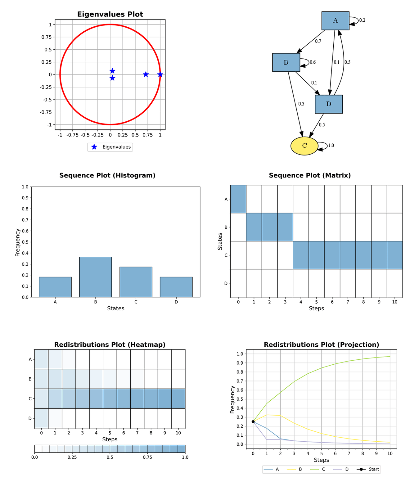
Below a few examples of MarkovChain plotting functions; in order to display the output of plots immediately, the interactive mode of Matplotlib must be turned on:

>>> plot_eigenvalues(mc, dpi=300)
>>> plot_graph(mc, dpi=300)
>>> plot_sequence(mc, 10, plot_type='histogram', dpi=300)
>>> plot_sequence(mc, 10, plot_type='heatmap', dpi=300)
>>> plot_sequence(mc, 10, plot_type='matrix', dpi=300)
>>> plot_redistributions(mc, 10, plot_type='heatmap', dpi=300)
>>> plot_redistributions(mc, 10, plot_type='projection', dpi=300)

Screenshots

Usage: HiddenMarkovModel Class

The HiddenMarkovModel class can be instantiated as follows:

>>> p = [[0.4, 0.6], [0.8, 0.2]]
>>> states = ['A', 'B']
>>> e = [[0.5, 0.0, 0.0, 0.5], [0.2, 0.2, 0.2, 0.4]]
>>> symbols = ['H1', 'H2', 'H3', 'H4']
>>> hmm = HiddenMarkovModel(p, e, states, symbols)
>>> print(hmm)
    
HIDDEN MARKOV MODEL
 STATES:  2
 SYMBOLS: 4
 ERGODIC: NO
 REGULAR: NO

Below a few examples of HiddenMarkovModel methods:

>>> sim_states, sim_symbols = hmm.simulate(12, seed=1488)
>>> print(sim_states)
['B', 'A', 'A', 'A', 'B', 'A', 'A']
>>> print(sim_symbols)
['H2', 'H4', 'H4', 'H4', 'H3', 'H4', 'H4']

>>> est_hmm = hmm.estimate(states, symbols, sim_states, sim_symbols)
>>> print(est_hmm.p)
[[0.75, 0.25]
 [1.00, 0.00]]
>>> print(est_hmm.e)
[[0.0, 0.0, 0.0, 1.0]
 [0.0, 0.5, 0.5, 0.0]]

>>> dec_lp, dec_posterior, dec_backward, dec_forward, _ = hmm.decode(sim_symbols)
>>> print(dec_lp)
-8.77549587
>>> print(dec_posterior)
[[0.00000000, 0.84422968, 0.41785105, 0.84422968, 0.00000000, 0.82089552, 0.52238806]
 [1.00000000, 0.15577032, 0.58214895, 0.15577032, 1.00000000, 0.17910448, 0.47761194]]
>>> print(dec_backward)
[[1.50000000, 0.88942581, 1.01307561, 0.79988630, 1.31154065, 0.94776119, 0.98507463, 1.00000000]
 [0.50000000, 1.00000000, 0.93462194, 1.21887436, 0.43718022, 1.00000000, 1.07462687, 1.00000000]]
>>> print(dec_forward)
[[0.50000000, 0.00000000, 0.83333333, 0.52238806, 0.64369311, 0.00000000, 0.83333333 0.52238806]
 [0.50000000, 1.00000000, 0.16666667, 0.47761194, 0.35630689, 1.00000000, 0.16666667 0.47761194]]

>>> pre_lp, pre_states = hmm.predict('viterbi', sim_symbols)
>>> print(pre_lp)
-13.24482936
>>> print(pre_states)
['B', 'A', 'B', 'A', 'B', 'A', 'B']

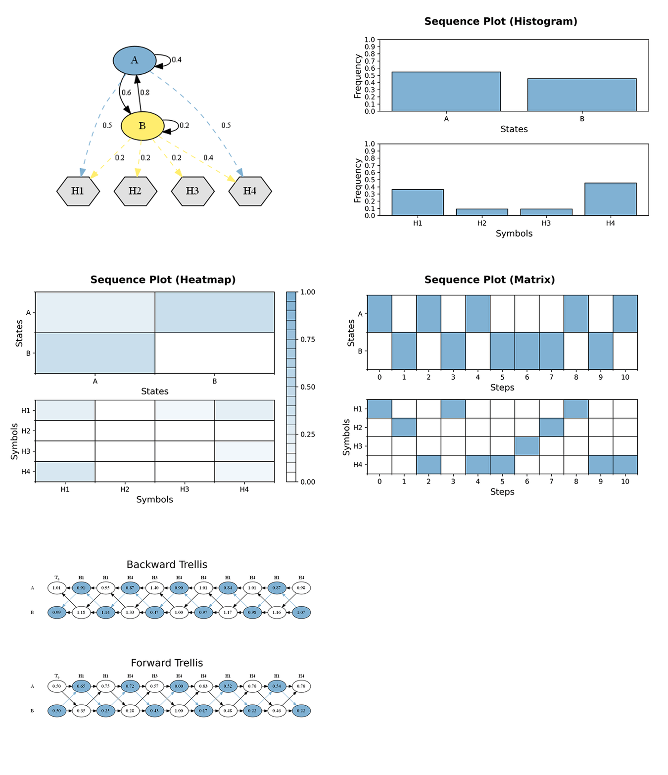
Below a few examples of HiddenMarkovModel plotting functions; in order to display the output of plots immediately, the interactive mode of Matplotlib must be turned on:

>>> plot_graph(hmm, dpi=300)
>>> plot_sequence(hmm, 10, plot_type='histogram', dpi=300)
>>> plot_sequence(hmm, 10, plot_type='heatmap', dpi=300)
>>> plot_sequence(hmm, 10, plot_type='matrix', dpi=300)
>>> plot_trellis(hmm, 10, dpi=300)

Screenshots

Metadata

Release files for PyDTMC 9.0.0

For a detailed explanation of source distributions (sdists) and built distributions (wheels), please see the package formats documentation.

Source distribution (sdist)

Source distribution for PyDTMC 9.0.0
File	Size	Uploaded
pydtmc-9.0.0.tar.gz	129.3 kB	Jul 5, 2026	Details

Built distribution (wheel)

Table of built distributions (wheels) for PyDTMC 9.0.0
File	Interpreter	ABI	Platform	Reset
pydtmc-9.0.0-py3-none-any.whl 76.5 kB Jul 5, 2026	Python 3	none	any	Details

Total release size: 205.9 kB

Release files / pydtmc-9.0.0.tar.gz

Download URL	pydtmc-9.0.0.tar.gz
Size	129.3 kB
Tags	Source
SHA-256 checksum How to use checksums	`e3cbe0e192bf85e1941b0b8b85314a5ae273df04aaa7c168667d0bb4fee5c8ef`
BLAKE2b-256 checksum How to use checksums	`13c14a705e08f64a2b23b386ebcbb5cd02b4bc7241ec3de8c96e91066a1a5b25`
Upload date	Jul 5, 2026
Uploaded using Trusted Publishing? What is trusted publishing?	No
Uploaded via	`twine/6.2.0 CPython/3.12.13`

Release files / pydtmc-9.0.0-py3-none-any.whl

Download URL	pydtmc-9.0.0-py3-none-any.whl
Size	76.5 kB
Tags	Python 3
SHA-256 checksum How to use checksums	`77ac6841f7ddd9423e9a2d1b7ab9c5c49bd0860f14d61dcc266d5e4b15c6420d`
BLAKE2b-256 checksum How to use checksums	`111f41a778f8687d74442d3d3f36b84fcda9273f3f2033b32b65189cb5413da5`
Upload date	Jul 5, 2026
Uploaded using Trusted Publishing? What is trusted publishing?	No
Uploaded via	`twine/6.2.0 CPython/3.12.13`