Sediment ANalysis & Deliniation through Images


Project description
 SANDI
SANDI
SANDI is a free, open-source software designed for oceanography and sedimentology. It can be used to extract suspended particles from high-resolution underwater images (on a single image or on a batch) and to extract gravels (> 1 mm) from a laboratory image, in order to measure their size and shape and to compute some statistics. Users can choose to download the full code and run the ‘main’ file, or they can download the latest release of the software as an executable, which is self-contained.
Disclaimer: This is an alpha version of the software, and it may therefore still contain some errors or malfunctions. In the TODO document, you can see the improvements planned for future versions, but any additional feedback or suggestion is welcome and appreciated, as we hope to make it a collaboratively improving tool.
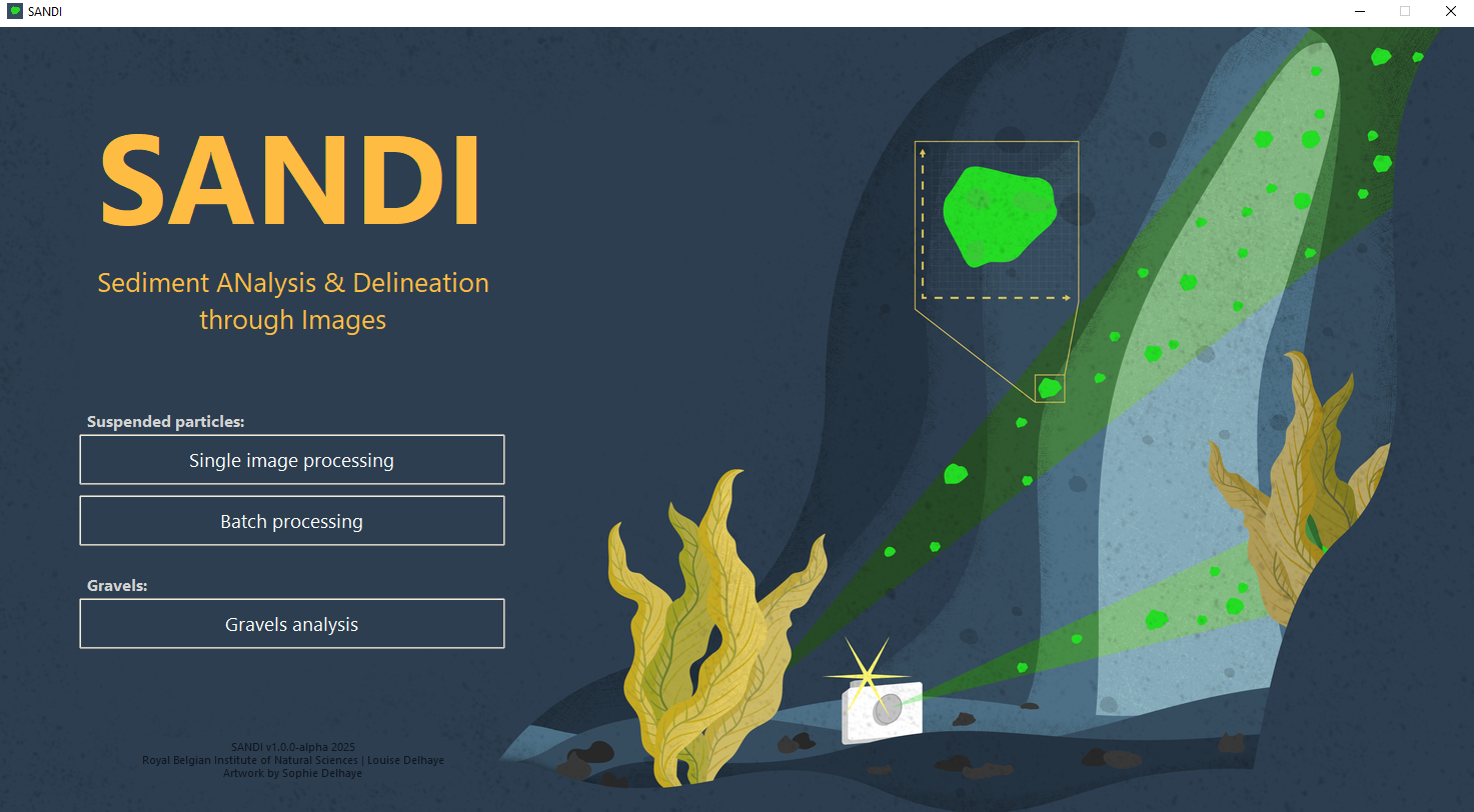
Figure 1. Homepage of the SANDI v1.0.0-alpha software. Artwork is from Sophie Delhaye.
1. Suspended particles
This section allows the user to process one or a batch of images of suspended particles and to extract their size and shape measurements. We strongly recommend that the user first processes a representative image from the batch in the ‘single image processing’ page in order to test which parameters' values for the image enhancement steps are best for each type of image and sample, as our tests have shown that these parameters can strongly influence the measured sizes and shapes. In the 'single image processing' page, the user has the possibility to test the effects of different values of these parameters on the resulting image and detected contours.
The 'single image processing' page contains a first frame on the left where the user can test the different image enhancement parameters, at the bottom of that frame, the 'extract particles' button allows the user to extract particles when the image is ready; and at the bottom left of the window, the histogram of the image is computed to help the user decide on the best parameters to enhance the image (Figure 2, left). That graph can be expanded. Once the image statistics are computed (see button on the right side of the window), this graph will be replaced by the computed particle size distribution. The imported image (and its modified version during the image enhancement process) is displayed at the center of the window, and at the bottom center, the console logs and details every step of the processing and results. The right side of the window contains options to filtrate the particles based on their intensity, size or aspect ratio; as well as two buttons to export the output csv files (after statistics computation) and vignettes. The algorithm was inspired by Markussen (2016).
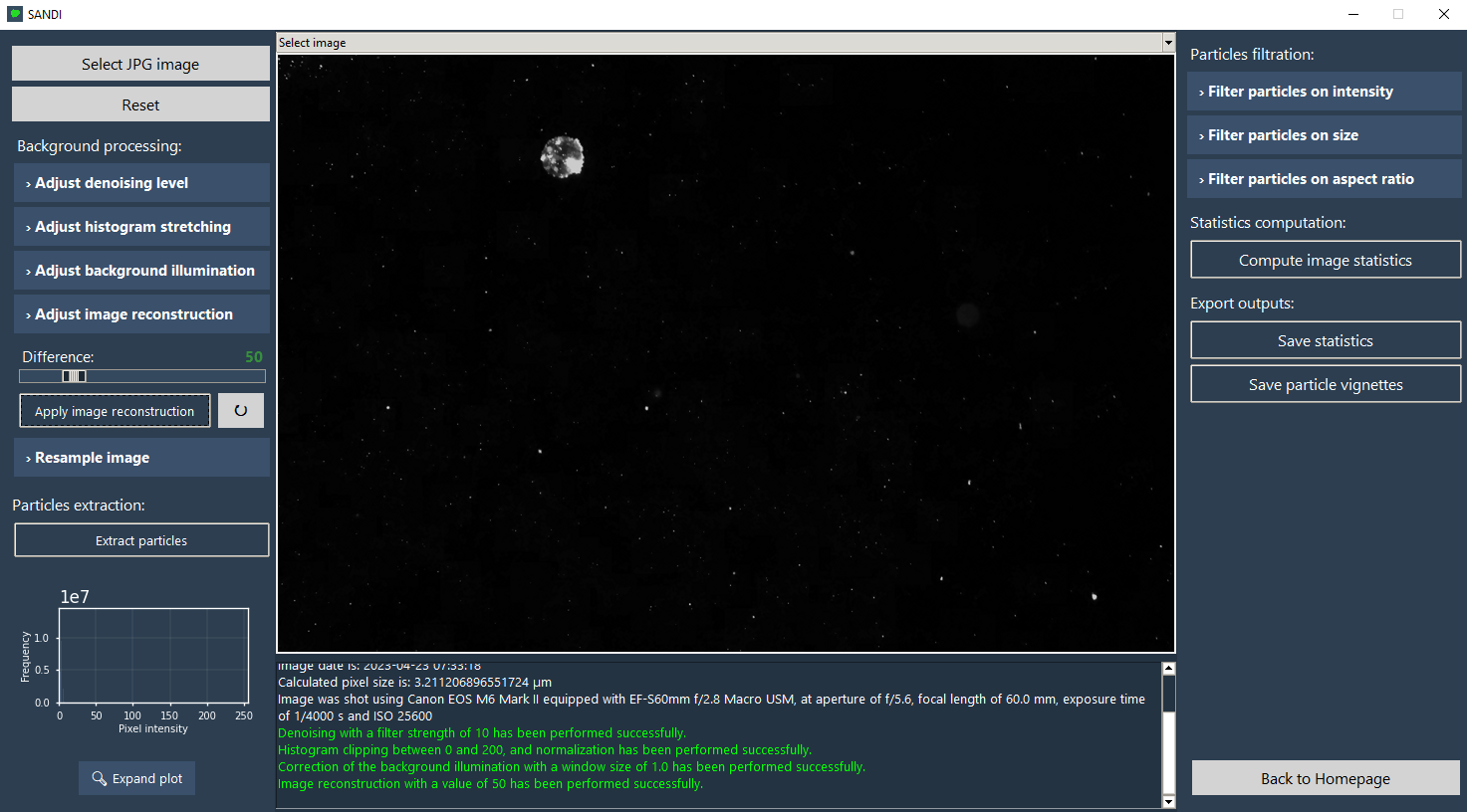
Figure 2. Demonstration of the single image processing page.
The 'batch processing' page allows the user to import a set of images, to define the desired image enhancement values (left frame) and to start the processing on the entire batch by clicking on the 'process batch' button on the top right corner of the window (Figure 2, right). Three new folders (corrected images, statistics and vignettes) will automatically be created in the directory chosen by the user which will contain the output results of the processing (enhanced images, csv files, graphs, log and individual vignettes of each particle). During the processing, the console logs and details all the steps of the processing, the top graph shows the particle size distribution updated with each new image from the batch processed and the bottom right graph shows the mean shape parameters of all the particles extracted in the batch.
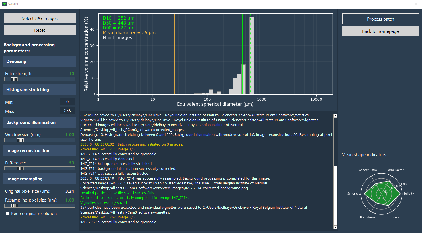
Figure 3. Demonstration of the batch processing page.
1.1. Input image
By clicking on the 'Select JPG image(s)' button, the user is invited to select one or multiples images to be processed. A pop-up should then appear allowing the user to insert the height, width and depth of field (in mm) of the images to be imported. The default values are for the PCam3 developed by Herbst Environmental Science. When clicking on the 'ok' button of the pop-up, the user should see the image appearing on the main window (only in the 'single image processing' page) and its name, date and metadata, as well as the calculated pixel size (in µm) should be written on the console below. Once the image is imported, the user has the possibility to measure a distance on the image by left-clicking and dragging a line.
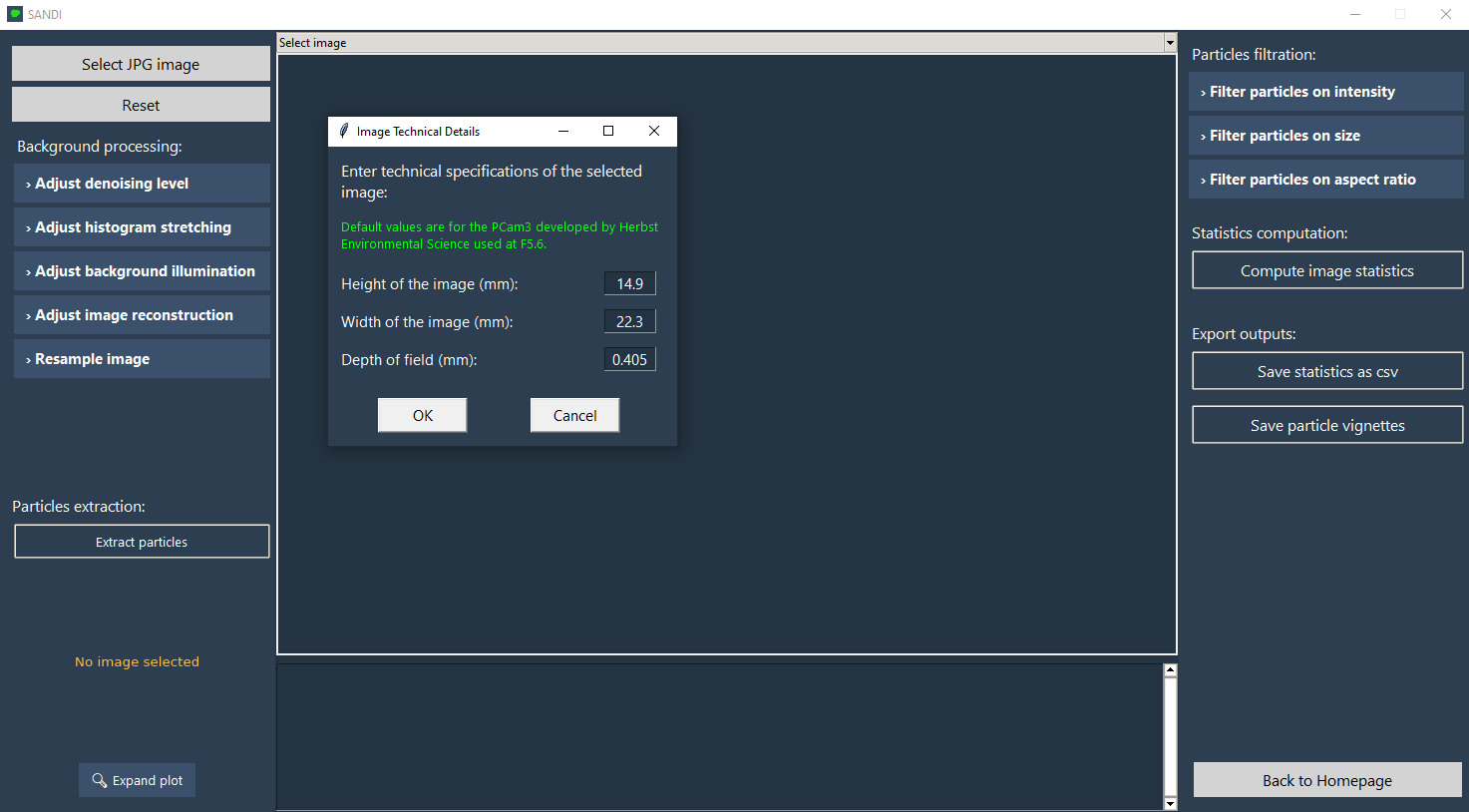
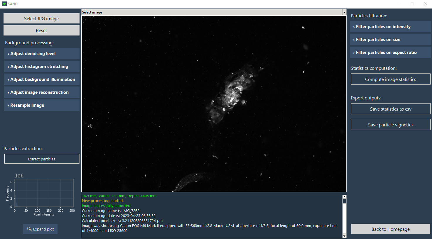
Figure 4. Demonstration of the windows when importing one or multiple image(s).
1.2. Image enhancement
Several steps are necessary to improve the contour detection of the particles on the image by enhancing the original image. These steps, on the left side of the page, are essential to obtain accurate size and shape measurements, they are briefly introduced here but further developed in Delhaye et al. (in prep). As mentioned earlier, it is highly recommended to test the effects of different values for each of these parameters on the final contour detection before processing a batch of images as the ideal values proved to be very specific to each type of particle. This can be done interactively on the 'single image processing' page.
1.2.1. Denoising
Using the Non-Local Means Denoising (NLMD) method from OpenCV, the denoising function of the software is designed to reduce the noise on the image. This step is recommended to improve shape indicators measurements as different factors (e.g. camera settings, environmental conditions) create noise in the image that can affect measurements. The user can manually adjust the denoising filter strength which will define the intensity of the denoising operation.
1.2.2. Histogram stretching
In this part, the user can adapt the minimum and maximum values of the image histogram (which is visible on the 'single image processing' page) in order to enhance the contrasts on the image.
1.2.3. Background illumination
The background illumination correction corresponds to the first part of to the “ImRec” function developed by Markussen (2016) and allows to homogeneize the background illumination in case some parts of the image are more illuminated than others. The size of the blocks (in mm) that are iterated over the image should be higher than the expected particle size.
1.2.4. Image reconstruction
The image reconstruction operation (corresponding to the second part of the “ImRec function of Markussen (2016)) performs morphological reconstruction on the image to enhance its features by selectively preserving or suppressing certain regions. The user can adjust the value to be substracted from the original image.
1.2.5. Resampling
The image resampling function adjusts the spatial resolution of the image to the one chosen by the user (set to 1 µm by default) by linearly interpolating the intensities of the four neighboring pixels of the selected pixel in order to find its new value. We recommend using this option to ensure all shape indicators are confined within the expected 0-1 range.
1.3. Particle extraction
Once these image enhancement operations are done, the contours of the particles are automatically extracted using the Otsu threshold. It creates a binary image that separates the particles from the background. As did Markussen (2016), the particles touching the border of the image are automatically discarded. Contours of every detected particle are then extracted from the image using functions from the scikit-image library in python. Upon clicking on the "extract particles" button, the user will see all the contours detected on the image on the screen and by hoving over with the cursor, the contours of the selected particle will be displayed on the bottom right side of the window, and a yellow pop-up will show the different values measured by the algorithm for that particle (see Figure below). By inspecting the results, the user can detect any abnormal value that may indicate that other settings should be used for the image enhancement. By right-clicking on a particle (or dragging a rectangle over multiple particles), the user can choose to discard one (or multiple) particles from the measurements. The process can be reversed by right-clicking on the image and selecting the 'restore particle(s)' option from the menu. This option as well as the visualization of the contours are only available in the 'single image processing' page and not in the 'batch processing' page.
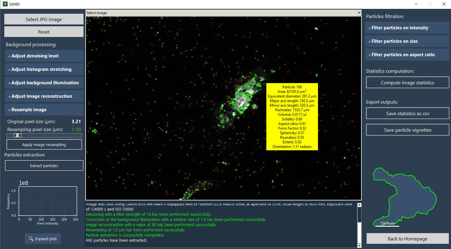
Figure 5. Demonstration of the extracted contours and particles measurements.
1.4. Particle measurements
For each extracted particle, the following measurements are computed:
- Area (in pixels and in µm)
- Equivalent spherical diameter (µm)
- Major and minor axis lengths (µm)
- Perimeter (µm)
- Euler number
- Solidity
- Form factor
- Volume (µl)
- Aspect ratio
- Sphericity
- Roundness
- Extent
- 2D fractal dimension (not yet in the executable)
- 3D fractal dimension (not yet in the executable)
- Mean pixel intensity (not yet in the executable)
- Kurtosis of the pixels intensity (not yet in the executable)
- Skewness of the pixels intensity (not yet in the exectuable)
For a more detailed explanation, the user is invited to read Delhaye et al. (in prep.).
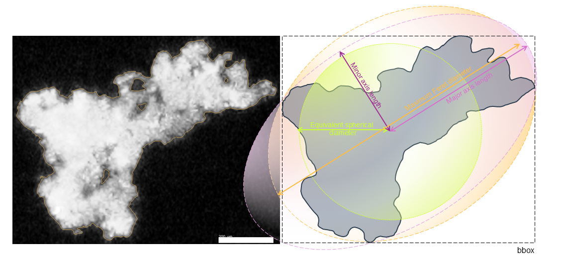
Figure 6. Representation of the core particle measurements, on which the size and shape metrics are based.
1.4. Statistics computation
The averages of each particle measurement for each image are calculated upon clicking on the 'compute image statistics' button, as well as the D10, D50 and D90. Results should be displayed in the console at the bottom of the window. The particles are grouped into 57 bins between 1 and 19144 µm based on their equivalent spherical diameter.
Note: The minimum reliable equivalent spherical diameter that can be detected with our reference camera (PCam3, 3.21 µm resolution) is of 10 µm (7 coherent pixels).
1.5. Outputs
The software generates two CSV files (the mean statistics and PSD of each image and one CSV containing the measurements of each particle in the image) as well as vignettes for each particle extracted showing its detected contours on the original image. It also creates a figure containing the PSD and the mean shape descriptors.
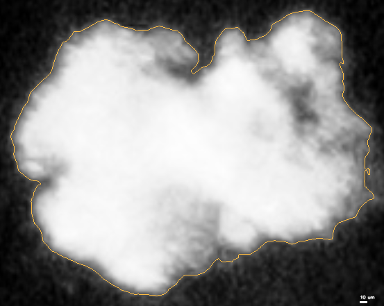
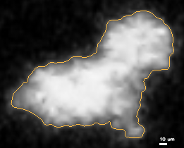
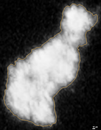
Figure 7. Examples of generated vignettes.
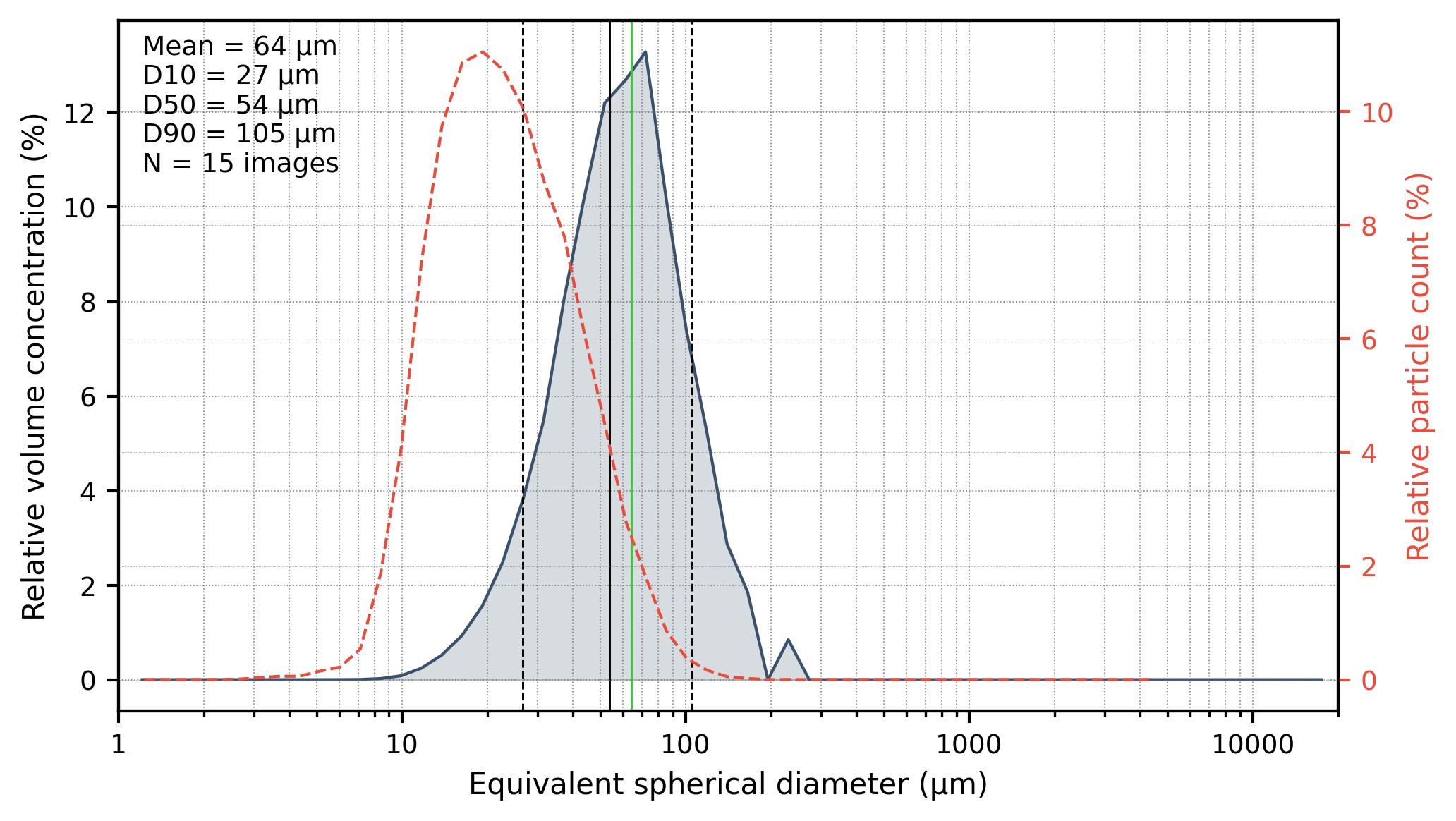
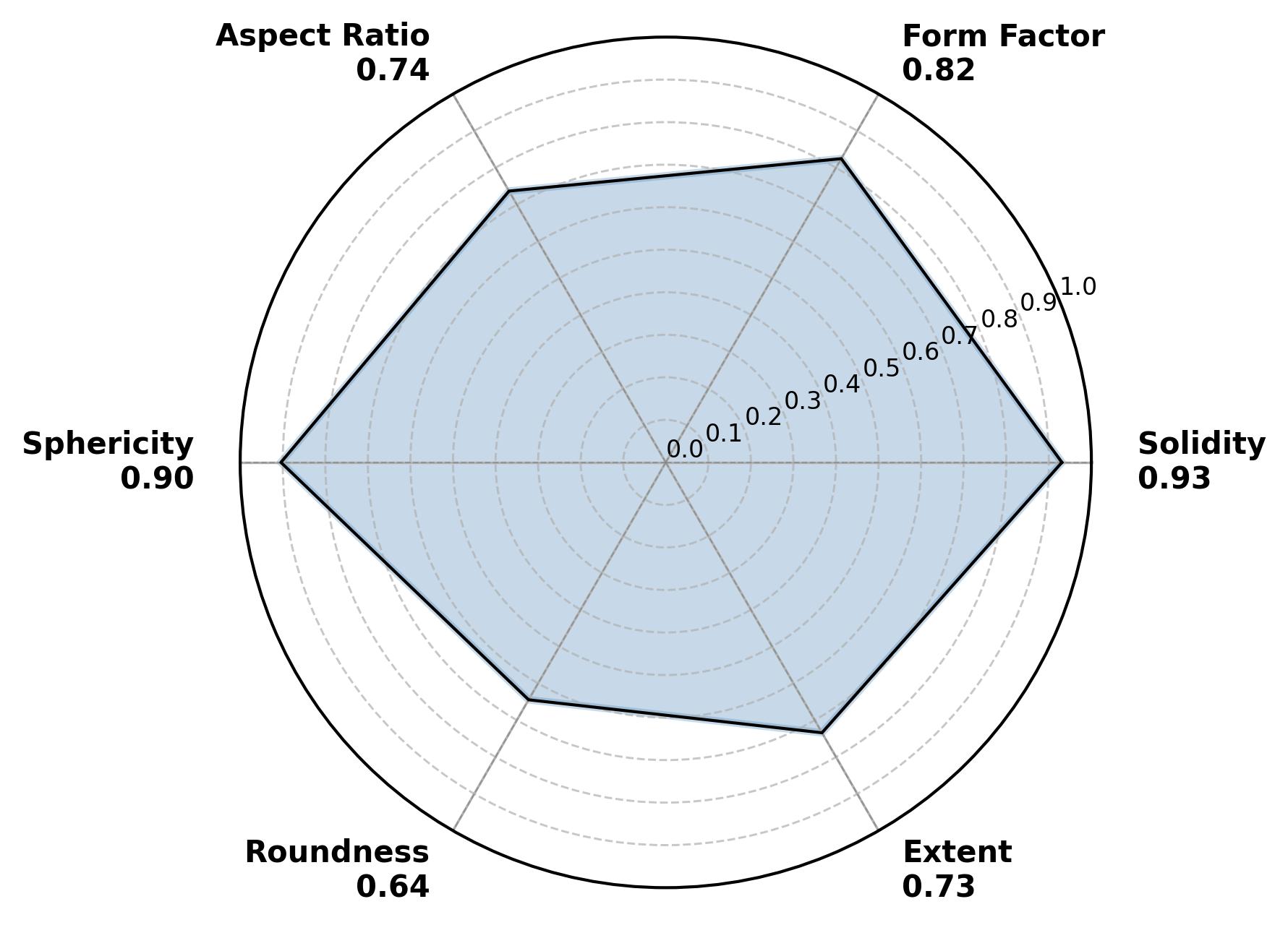
Figure 8. Output figures.
2. Gravel analysis
This section presents a fast and easy way to measure the size and shape of rocks by detecting their contours from an image taken in a laboratory. The beta version of this section is still under construction. Although it already is operational, it still has potential for improvement. Please bear this in mind when using it.
2.1. Input image
The input image should contain the rocks displayed on a white or green background (see two options later), together with a ruler and a label. The image should be shot from above in order to have a good overall vision of the samples and to avoid measurement inaccuracies due to changes in the image geometry. We recommand using a green background for rocks with a light or a wide range of colors, and a white background for darker gravels. The contour detection is very sensitive to lighting and shadows, we therefore recommand to photograph the samples with sufficient, homogenous natural light, that generates as little shadow as possible. If the details of the rocks extracted are important, we recommend using a camera specially designed for macro shots, that will highly improve the quality of the vignettes.
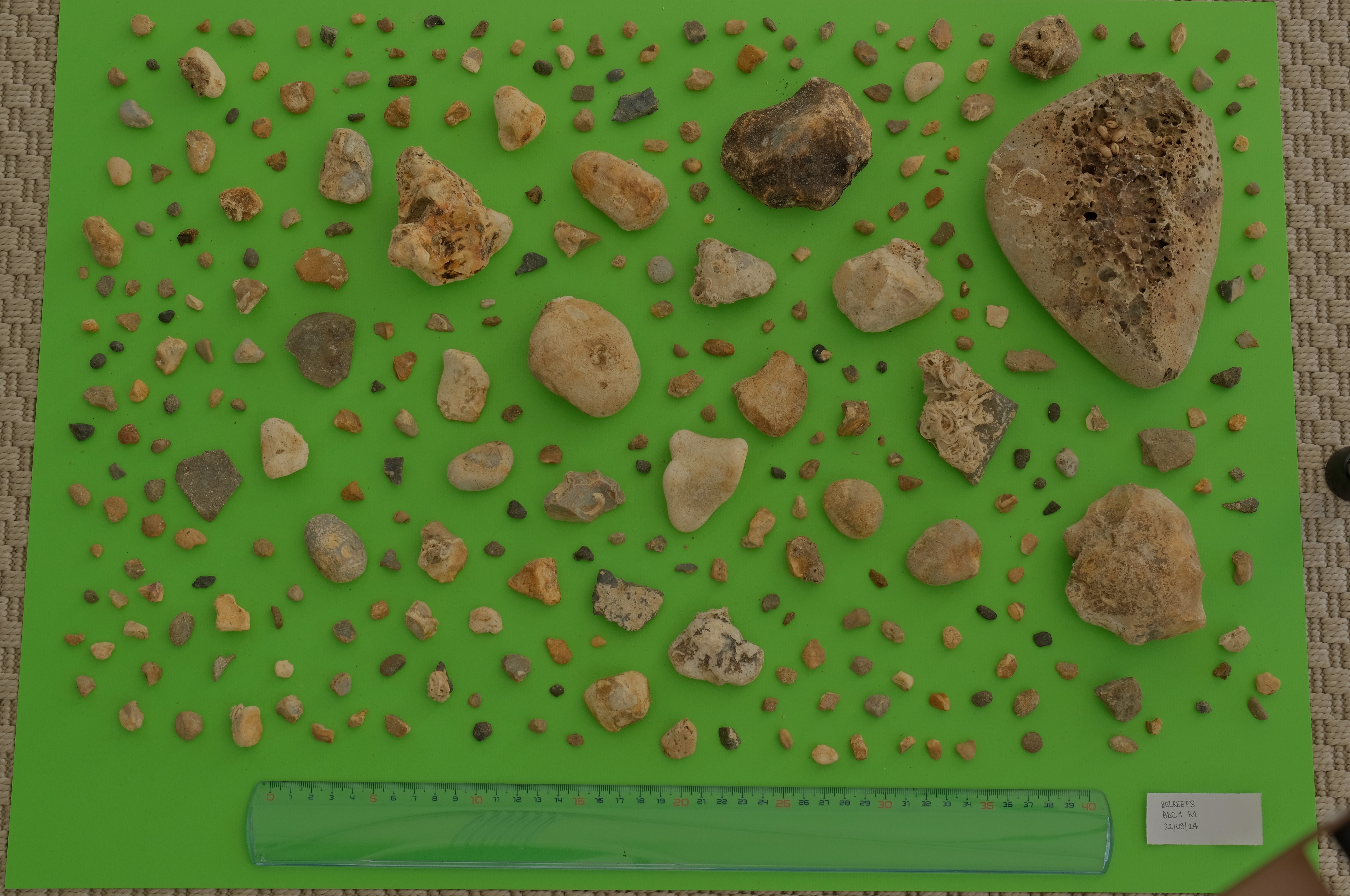
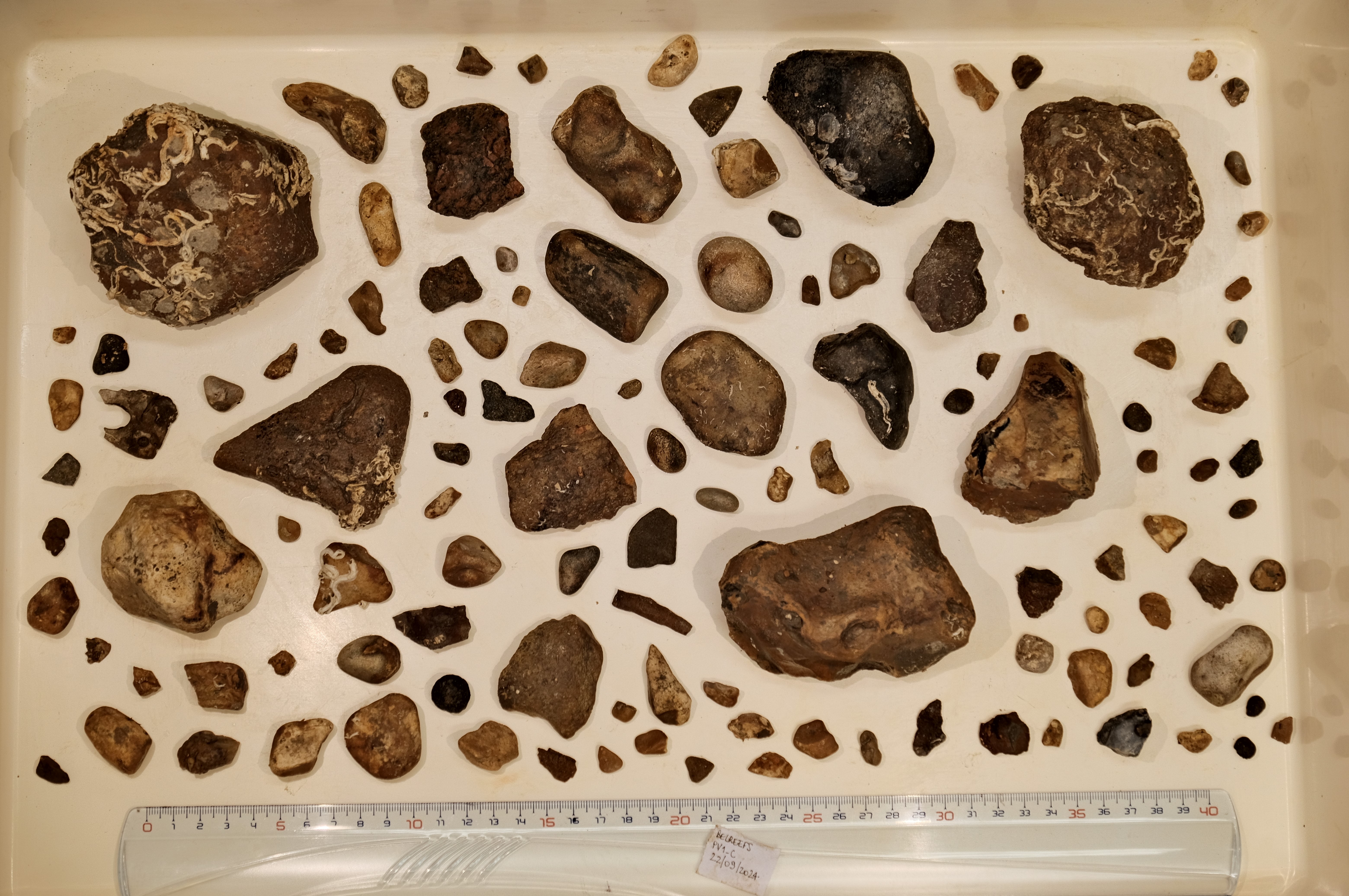
Figure 9. Examples of input images on a green and on white background.
2.2. Scale measurement
When the images in jpg are imported in the software, the user is invited to draw a line representing one centimeter on the ruler displayed on the picture, enabling the software to calculate the scale of the image. The accuracy of this measurement is essential for the reliability of the results that are calculated based on the measured pixel size, so we recommend drawing the line several times in order to see the variability and compare the different pixel sizes obtained each time. A value can be considered correct when it is measured several times. For better accuracy, we recommend that the ruler is aligned parallel to the edge of the image.
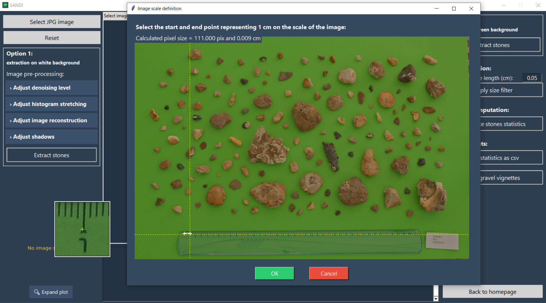
Figure 10. Demonstration of the scale definition.
2.3. Background correction: white background image
In the case of an image with a white background, defining a threshold can be complicated, particularly if the samples photographed contain stones of different colours, including light colours that are easily mistaken for the background. In such cases, different processes for enhancing the original image can be applied to obtain better results. The different enhancement methods can be found in the frame "Option 1" in the software, see green rectangle on the image below.
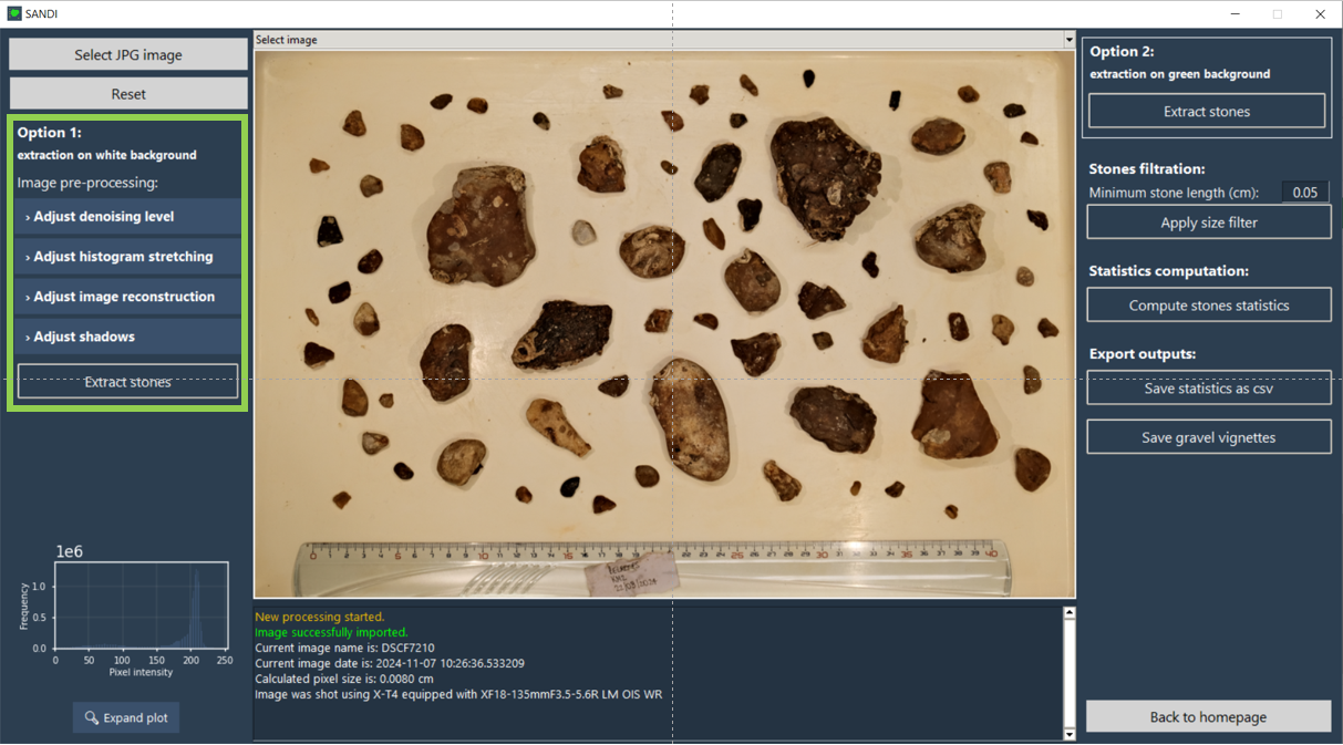
Figure 11. Localisation of the options to enhance the image on a white background in the software (see frame highlighted in green).
2.3.1. Denoising
The denoise function is designed to reduce noise in a grayscale image using the Non-Local Means Denoising method from OpenCV. The strength of the denoising filter can be adjusted manually by the user but is set to 15 by default, which after trial and errors showed to be the best fit for our test images. Performing this operation is essential to obtain representative shape indicators as noise on the image incorrectly increases the complexity of the edges of detected objects (see Figure 9).
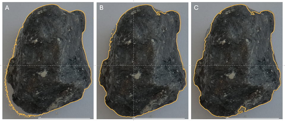
Figure 12. Impact of different values of the denoising filter strength (A: 0; B: 15; C: 30).
2.3.2. Histogram stretching
The histogram stretching operation is used on the greyscale image to clip the pixel intensity values within a specified range and then stretch the resulting values to cover the full 8-bit range (0–255). It allows to enhance the contrasts on the image.
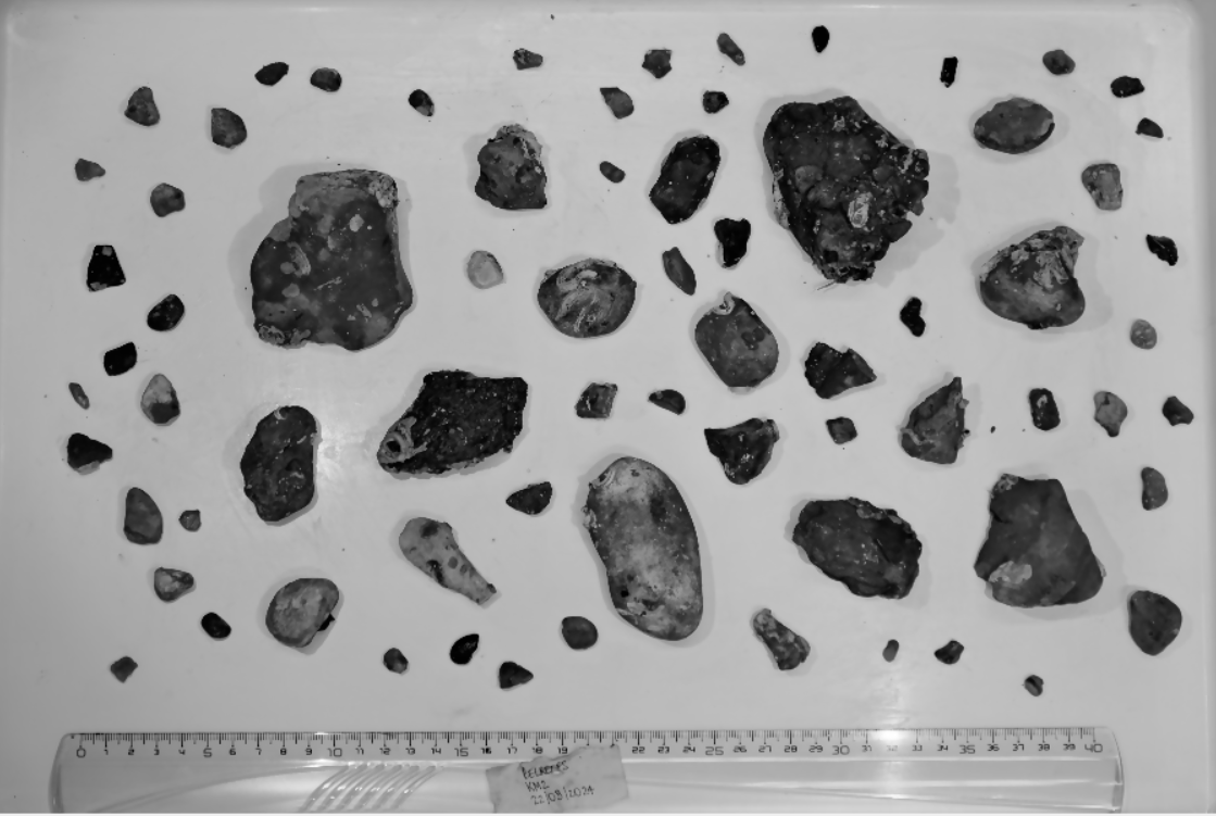

Figure 13. Impact of the histogram stretching (left: no histogram stretching; right: histogram stretched between 0 and 200).
2.3.3. Image reconstruction
The image reconstruction operation helps keeping important objects on the image while removing unwanted ones. It works bu using two versions of the image: the mask and the marker. While the mask consists of the original image, the marker is the original image in which each pixel's intensity is reduced by a certain value - which is decided by the user. In that new image, all the pixels which intensities become lower than the threshold are set to 0. Through the reconstruction process, the marker image is gradually increased by a method called "dilation" so that no pixel in the new image has an intensity higher than its intensity in the mask image. This technique is useful for making objects clearer, improving their shapes and removing unwanted noise from the image.

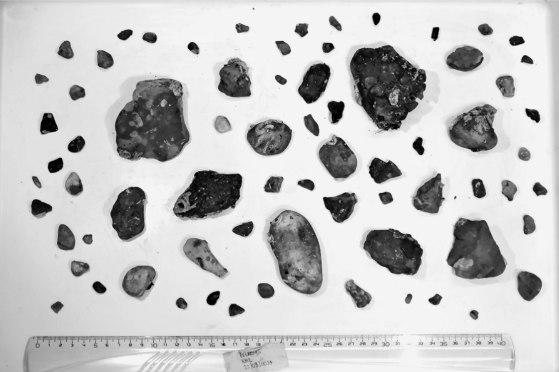
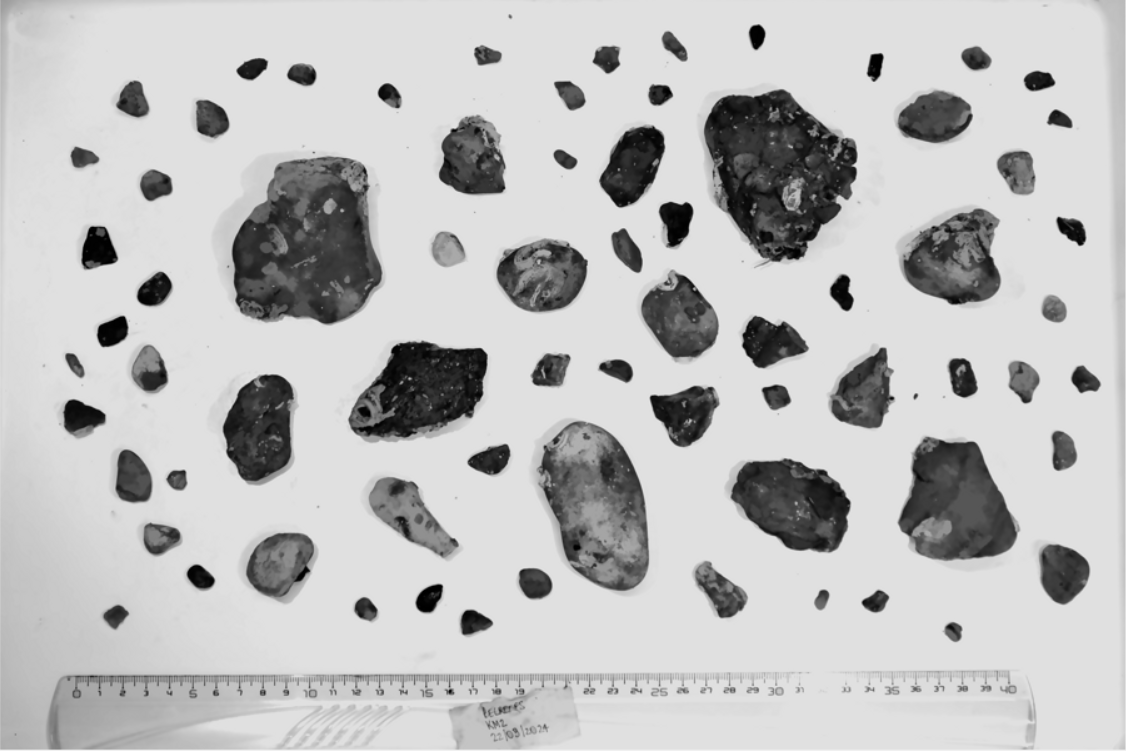
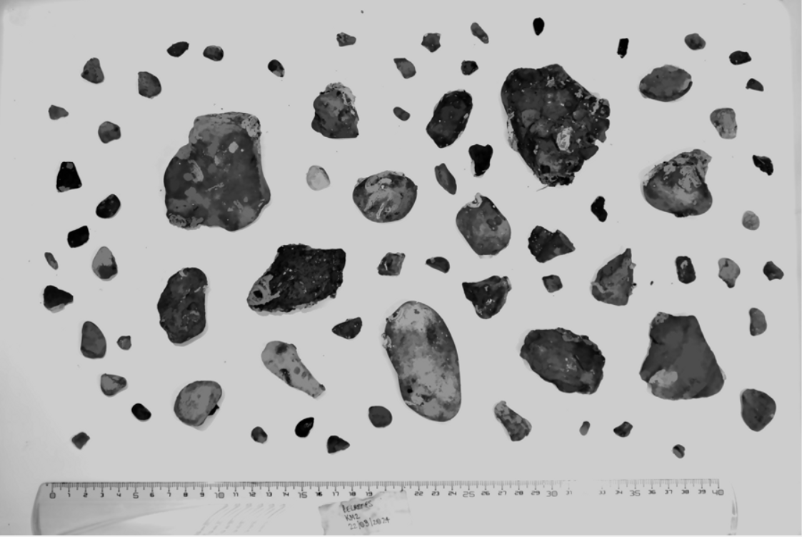
Figure 14. Impact of the value used in the reconstruction (upper left: no image reconstruction; upper right: image reconstruction with a difference of 10; lower left: image reconstruction with a difference of 30; lower right: image reconstruction with a difference of 50).
2.3.4. Shadow correction
The gamma correction allows to adjust the brightness and contrast of the image. Instead of changing all pixels equally, it applies a special curve that makes dark areas (shadows) brighter (with gamma value < 1) or bright areas darker (with a gamma value > 1).

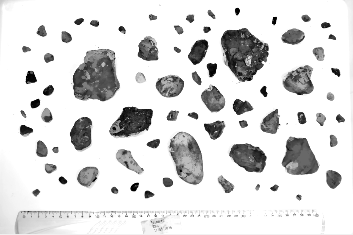
Figure 15. Impact of the gamma correction (left: no gamma correction ; right: gamma correction at 0.9).
2.4. Contours detection and gravel extraction
2.4.1. For an image with a white background
For an image with a white background, the objects are detected after converting the enhanced image to binary using the Otsu thresholding method. Objects touching the borders of the image are then removed and holes inside detected objects are filled using morphological closing and binary holes filling. Finally, each object is labelled and its properties are extracted using the regionprops function from skimage. For more information regarding the different measurements made, we advise the user to refer to the corresponding section in the suspended sediment part of this guide.
2.4.2. For an image with a green background
For an image with a green background, the objects are detected after a first denoising (Non-Local Means) is applied to the original HSV image. The background is then detected by creating a mask on a specified range of color (corresponding to the green of the background), effectively converting these pixels to white. The mask is then inverted, isolating the gravels from the background. As for the image with a white background, objects touching the borders of the image are then removed and holes inside detected objects are filled using morphological closing and binary holes filling. Each object is labelled and its properties are extracted using the regionprops function from skimage. For more information regarding the different measurements made, we advise the user to refer to the corresponding section in the suspended sediment part of this guide.
2.5. Gravel filtration
Whatever the background chosen, this method will also detect objects that are not the gravels of interest (e.g. the ruler, label, little fragments of stones). These can be removed manually by the user by right-clicking or dragging a rectangle near the centroid(s) of the object(s) to be discarded, and recovered afterwards if needed. There is also an option for the user to remove all gravels under a desired size (cm).
2.6. Statistics computation
Once the unwanted objects have been removed from the image, the user can press the ‘Compute statistics’ button on the right side of the window. This will compute the mean area (cm²), perimeter (cm), equivalent spherical diameter (cm), major and minor axis lengths (cm), shape indicators and will aggregate the detected objects in bins of 0.1 cm based on their minor and major axis lengths and count the number of gravels per class on the GRADISTAT classification. It will also compute the sorting, skewness and kurtosis values of the sample.
2.7. Outputs
Finally, the user can save the vignettes of each detected gravel in png and export the individual properties of each gravel as well as the statistics of the entire sample in two separated csv files. Three graphs are saved in the same folder, one showing the gravel size distribution, the percentage of each GRADISTAT class and the mean shape indicators of the sample (see images x and x).
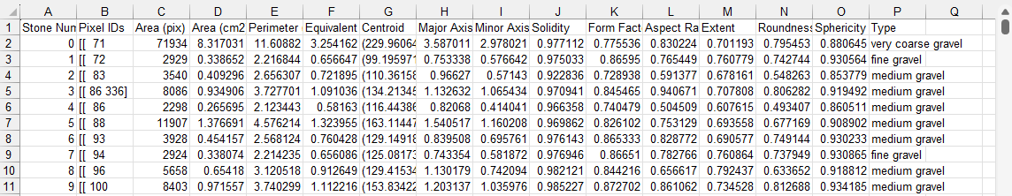
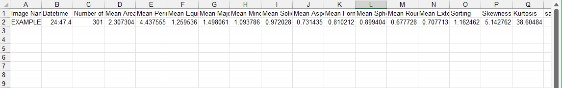
Figure 16. Examples of the two csv created (left: the measurements of each gravel on the image; right: the mean statistics for the entire image).
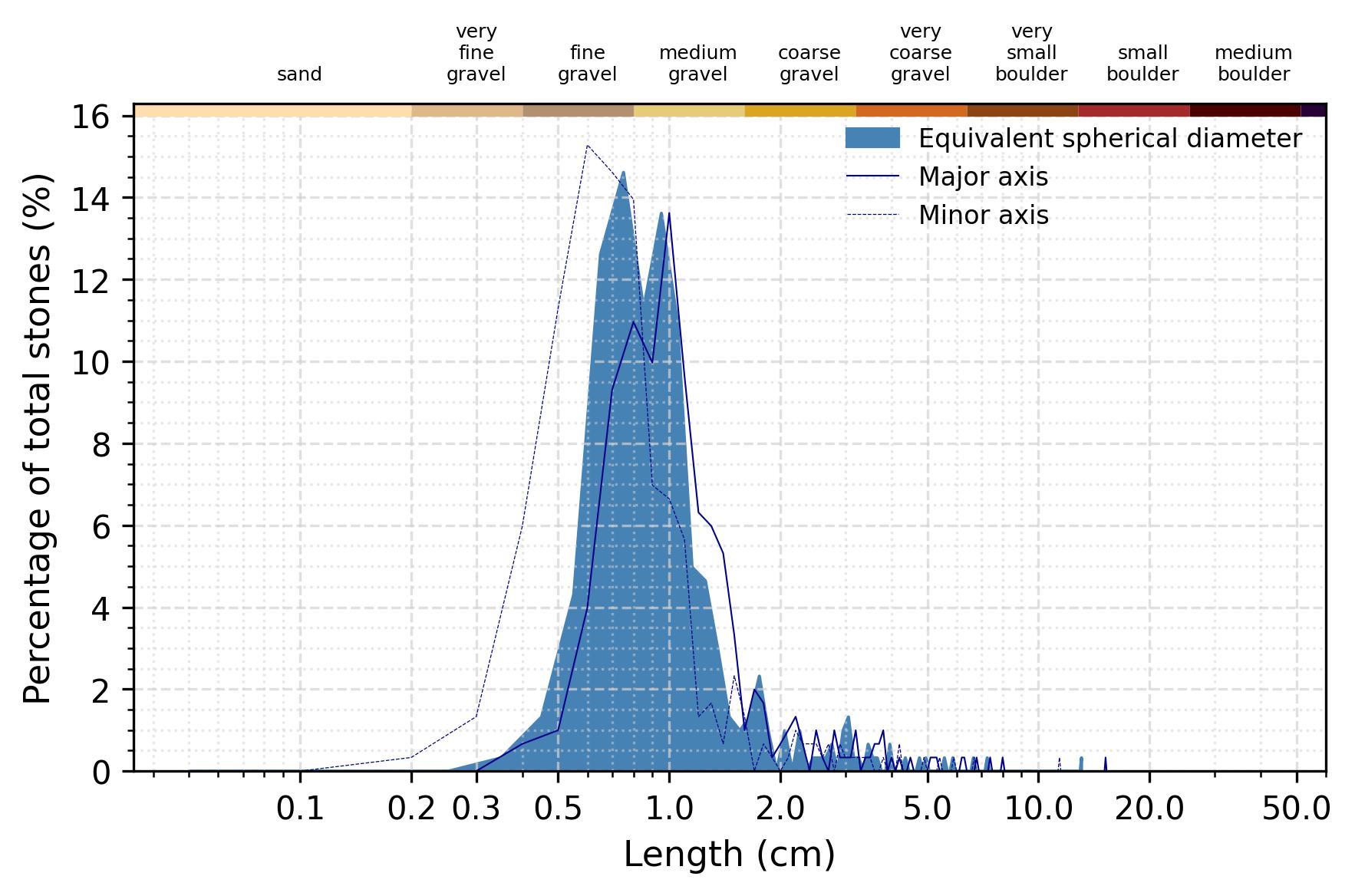
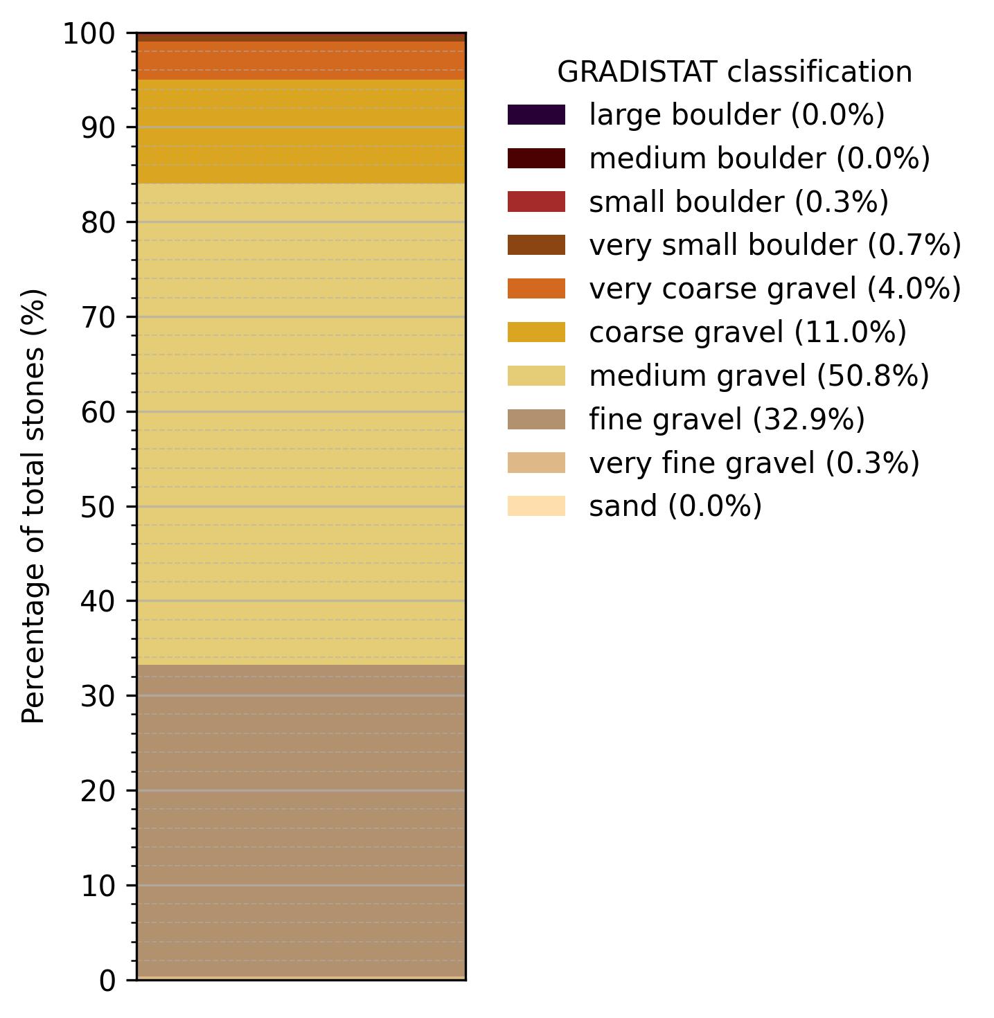
*Figure 17. Example of generated gravel size distribution and GRADISTAT classification of the gravels *
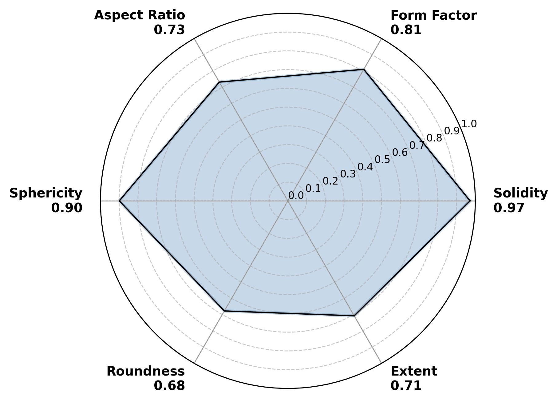
Figure 18. Example of generated mean shape indicators figure
2.8. Examples of shape indicators
Hereunder are shown a few gravels and their derived shape indicators as a reference for the user.
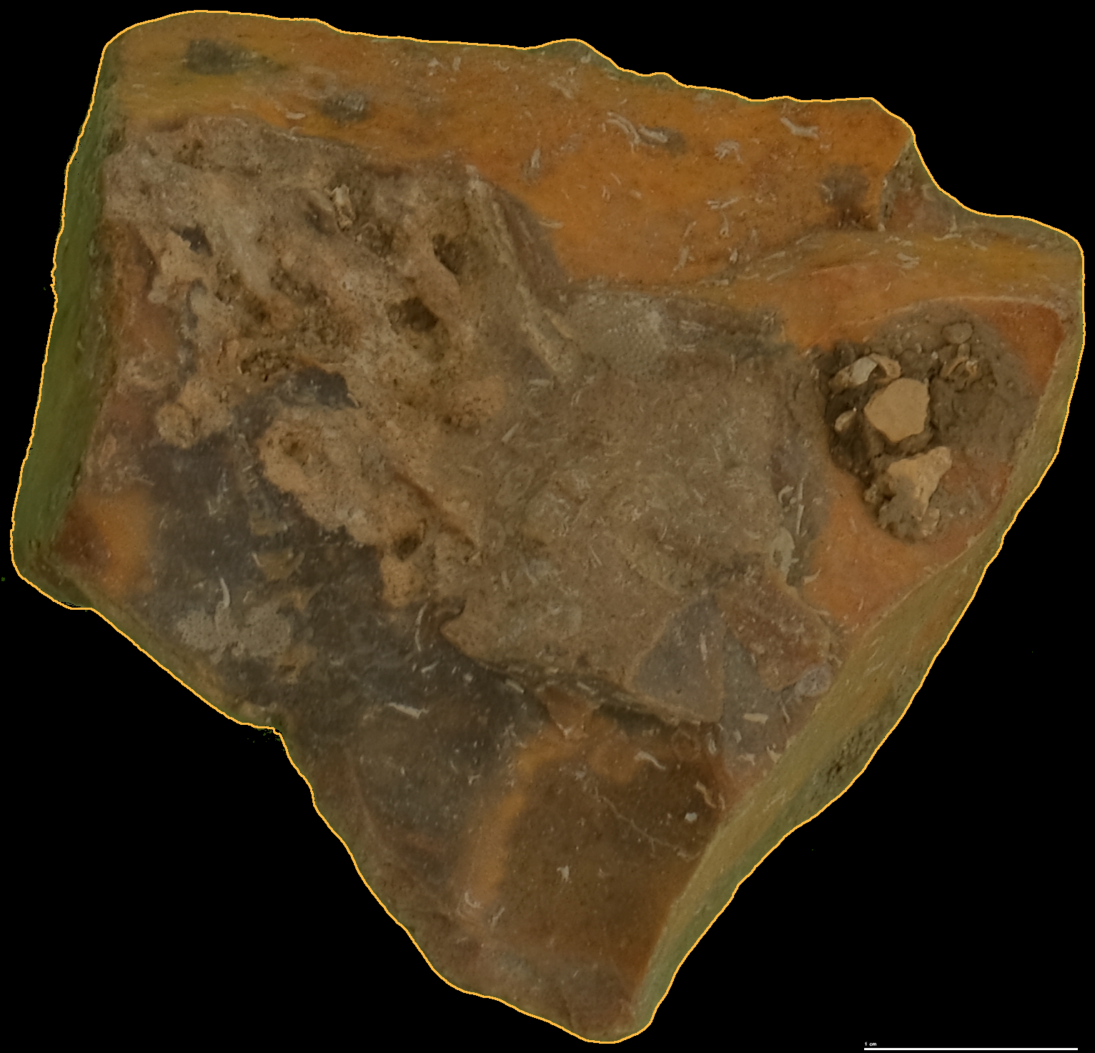
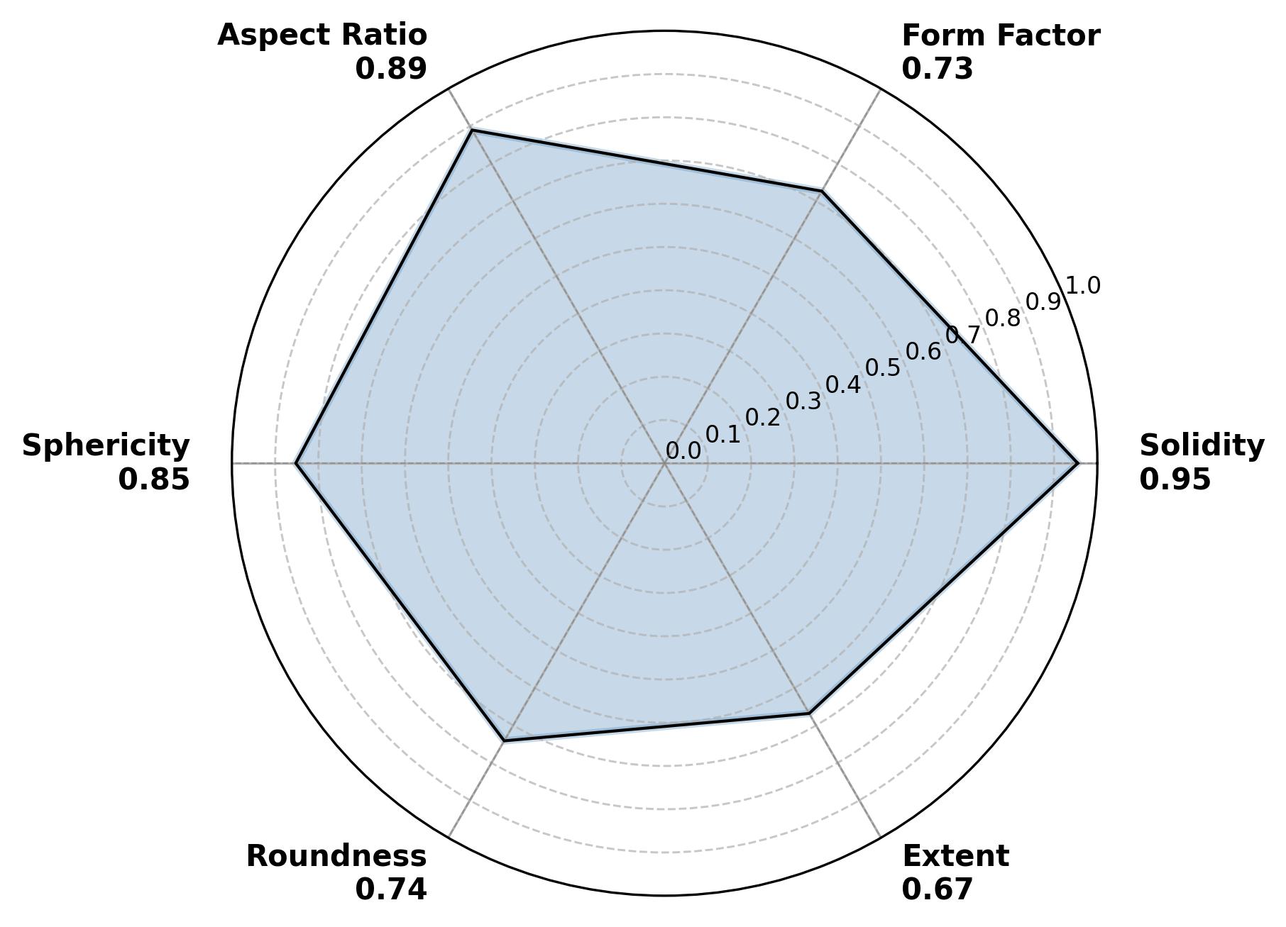
Figure 19. Example of angular stone.
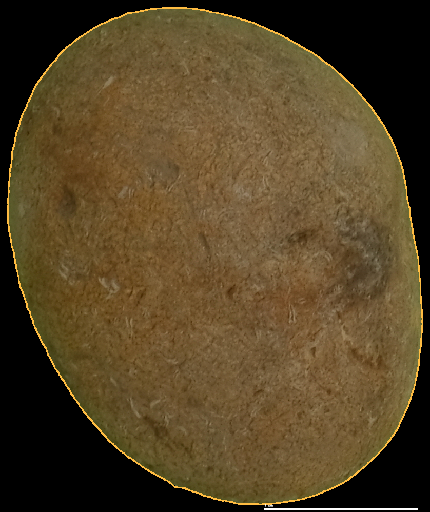
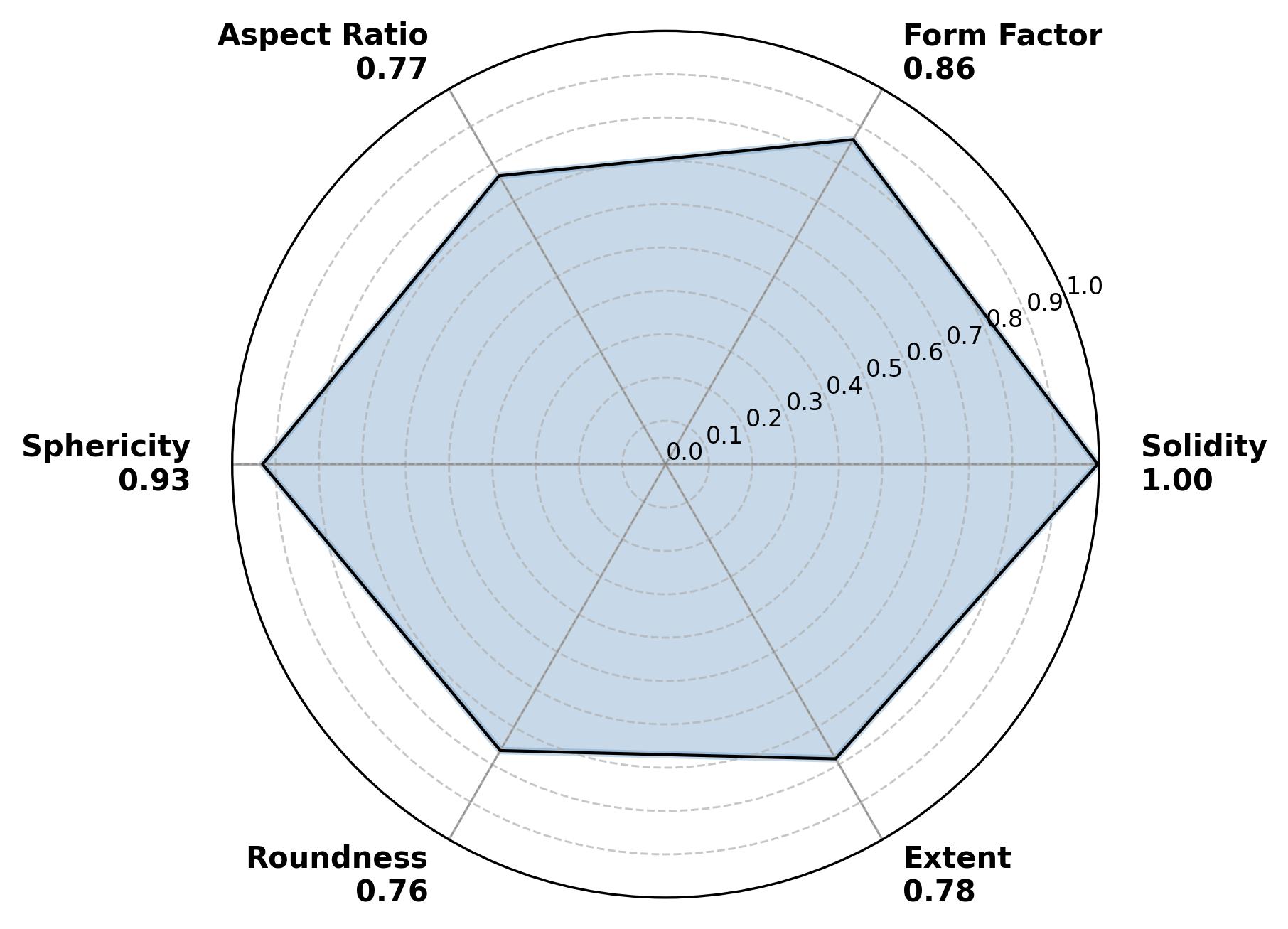
Figure 20. Example of rounded stone.
3. References
Markussen T.N., 2016. “Parchar - Characterization of Suspended Particles Through Image Processing in Matlab”, Journal of Open Research Software 4: e26. http://dx.doi.org/10.5334/jors.114.


Download files
Download the file for your platform. If you're not sure which to choose, learn more about installing packages.
Source Distribution
Built Distribution
Filter files by name, interpreter, ABI, and platform.
If you're not sure about the file name format, learn more about wheel file names.
Copy a direct link to the current filters
File details
Details for the file sandi-0.1.3.tar.gz.
File metadata
- Download URL: sandi-0.1.3.tar.gz
- Upload date:
- Size: 100.4 kB
- Tags: Source
- Uploaded using Trusted Publishing? No
- Uploaded via: twine/6.1.0 CPython/3.11.13
File hashes
| Algorithm | Hash digest | |
|---|---|---|
| SHA256 |
2dd46c081e608f65ee890e912f1af57f3f608a3a4d3f6891d318ca54d2997bf6
|
|
| MD5 |
23a57805f1b32d6787a73ea4e04954e3
|
|
| BLAKE2b-256 |
6b6b3528ccc7358d8bd7e3e06900e8890fa5ad9044b87d49f78c557526bfaca6
|
File details
Details for the file sandi-0.1.3-py3-none-any.whl.
File metadata
- Download URL: sandi-0.1.3-py3-none-any.whl
- Upload date:
- Size: 105.5 kB
- Tags: Python 3
- Uploaded using Trusted Publishing? No
- Uploaded via: twine/6.1.0 CPython/3.11.13
File hashes
| Algorithm | Hash digest | |
|---|---|---|
| SHA256 |
a52086b5bd867a9b227e64584e67957bfa9c0b886861fda362350c4d1b11f521
|
|
| MD5 |
bd875148f474efefe43c427f2213a2e8
|
|
| BLAKE2b-256 |
0994ec49a9371e5c59be69cfbc6d6088721dab798346487d23323cdd010150c7
|


