
ARPES viewer




Version 1.3.3 (last modified 10 November 2026) -- what changed is in CHANGELOG.md. For non-commercial use only; see the terms of use.
A Python/PyQt5 program for ARPES data: browse the measurements of a beamtime, open them in their own windows, convert to momentum, cut, fit, process, compare with a band-structure calculation, and lay the results out as a publication figure.
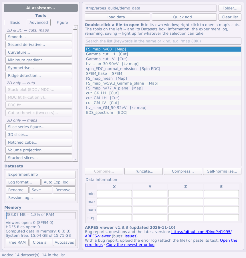
A note from the author on AI agents. Talking with beamline users, I heard two concerns again and again: running an AI agent on local data is unfamiliar, and the data might end up with an AI company and be used for training. The AI assistant panel (top of the tool panel) is my answer to the first. Choose the data folder and the results folder, tick a few options, and it writes the prompt to paste into your AI app. No configuration and no manual to read first. Every step the agent runs is listed with its code and output, a status light shows its state, and Pause hands the controls back to you at any time (how it works). On the second concern: the raw data files stay on your computer and are processed there. What the agent reads is sent to the AI provider as part of the conversation: printed results, fitted values, and the pictures it inspects to judge a step. Whether that is used for training depends on your provider and your account settings, so check them. Keep private code out of any folder the agent can reach. In my view, AI in ARPES experiments and analysis is here to stay. An experiment update prepared by the agent, which you check step by step, is a low-risk way to get familiar with it.
What it does
- Reads SOLEIL ANTARES and CASSIOPEE, ALS MAESTRO, ALBA LOREA, Diamond I05 and I05-1, MAX IV Bloch, Elettra APE, BESSY One Cube / One Square, SOLARIS URANOS, ASTRID2 SGM4, and its own saved format (loading data).
- Shows cuts, Fermi-surface maps, photon-energy scans, spatially resolved scans and spin-resolved curves, each in its own window with linked cursors (the viewers).
- Converts maps and cuts to momentum, photon-energy scans to k_z, with the Brillouin zone drawn over them (§4.8, §4.9–4.10, §4.11).
- Analyses: Fermi-edge fits, Fermi-surface correction, MDC / EDC fits and the self-energy, ridge detection, curvature, second derivatives and the minimum gradient, dichroism, core levels, spin, de-gridding, detector corrections, and the Fermi pockets of quasi-two-dimensional samples (under test) (Parts 3–5).
- Compares with theory: crystal structures, tight-binding fits, and calculated bands from Wien2k, VASP, Quantum ESPRESSO, Wannier90 and the FPLO + Wannier tools -- along a path, as constant-energy contours on any (hkl) plane, or as a 3-D Fermi surface (§6.2–6.5).
- Makes figures: the figure composer, laid out like a manuscript page, exported as PNG, PDF or SVG, and saved with its data (§6.1, 6.6).
- Loses nothing: every derived dataset is autosaved, a crash is recovered from, and long steps show a progress bar (§8.1).
Installing and starting
Needs Python 3.9+. With pip, which installs PyQt5, pyqtgraph, numpy, h5py and scipy with it:
pip install arpes-viewer
arpes-viewer
(python -m arpes_viewer does the same; for the latest, unreleased
version: pip install git+https://github.com/DingPei1995/ARPES-viewer.)
From a downloaded copy of this repository, with those packages installed:
python ARPES_viewer.py
- Windows: double-click
ARPES viewer.pywin this folder: no console window to close by mistake (the output goes to~/.arpes_viewer/launcher.log). - macOS: double-click
ARPES viewer.appin this folder. It finds a Python that has the packages (conda included), remembers it, and says what to install if none has. The first time, if macOS calls it an app from an unidentified developer: System Settings → Privacy & Security → Open Anyway. - No beamtime at hand?
python devtools/demo_data.pywrites the synthetic demo data of the example figures below todemo_data/(trying it with demo data).
From raw data to a publication figure
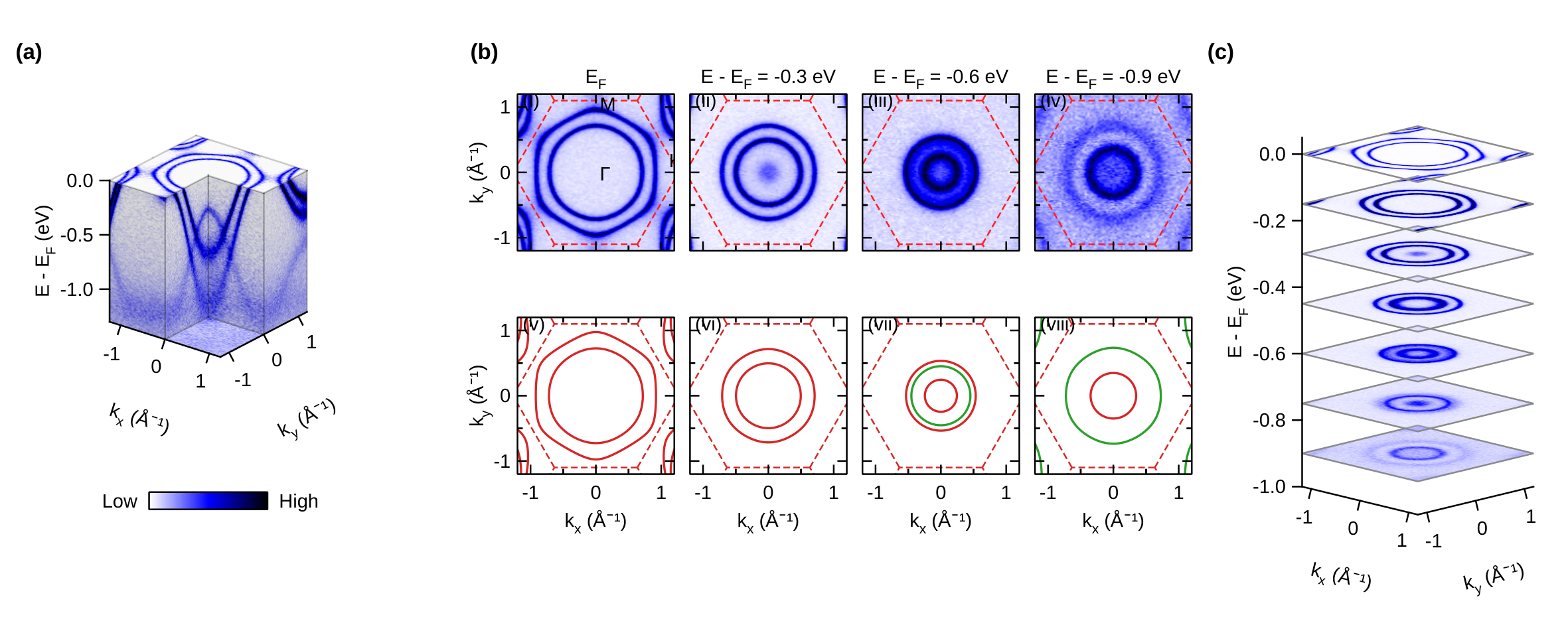
These are not real experimental data. Every panel above is made from the program's synthetic demo data (
devtools/demo_data.py): an invented tight-binding toy model -- a triangular lattice, a = 3.3 Å, stacked with c = 6 Å, a few bands with orbital labels and a k_z dispersion -- turned into spectra with a Fermi-Dirac cut-off, the analyser resolution and Poisson counting noise, and written as beamline files. The "calculation" in panel (b) is the same toy Hamiltonian made deliberately 1/0.8 times wider and 50 meV higher, so that comparing it with the "measurement" has something to find. No published data or literature were used to generate them: the model and its parameters are invented, and names such as "Se-pxy" or "1T-TiSe₂-like" are labels for the toy, not a description of a real material. (The only tabulated values in the demo set are the X-ray line energies of its synthetic EDS spectrum, standard emission energies as listed in the X-ray Data Booklet; that spectrum is not part of this figure.)
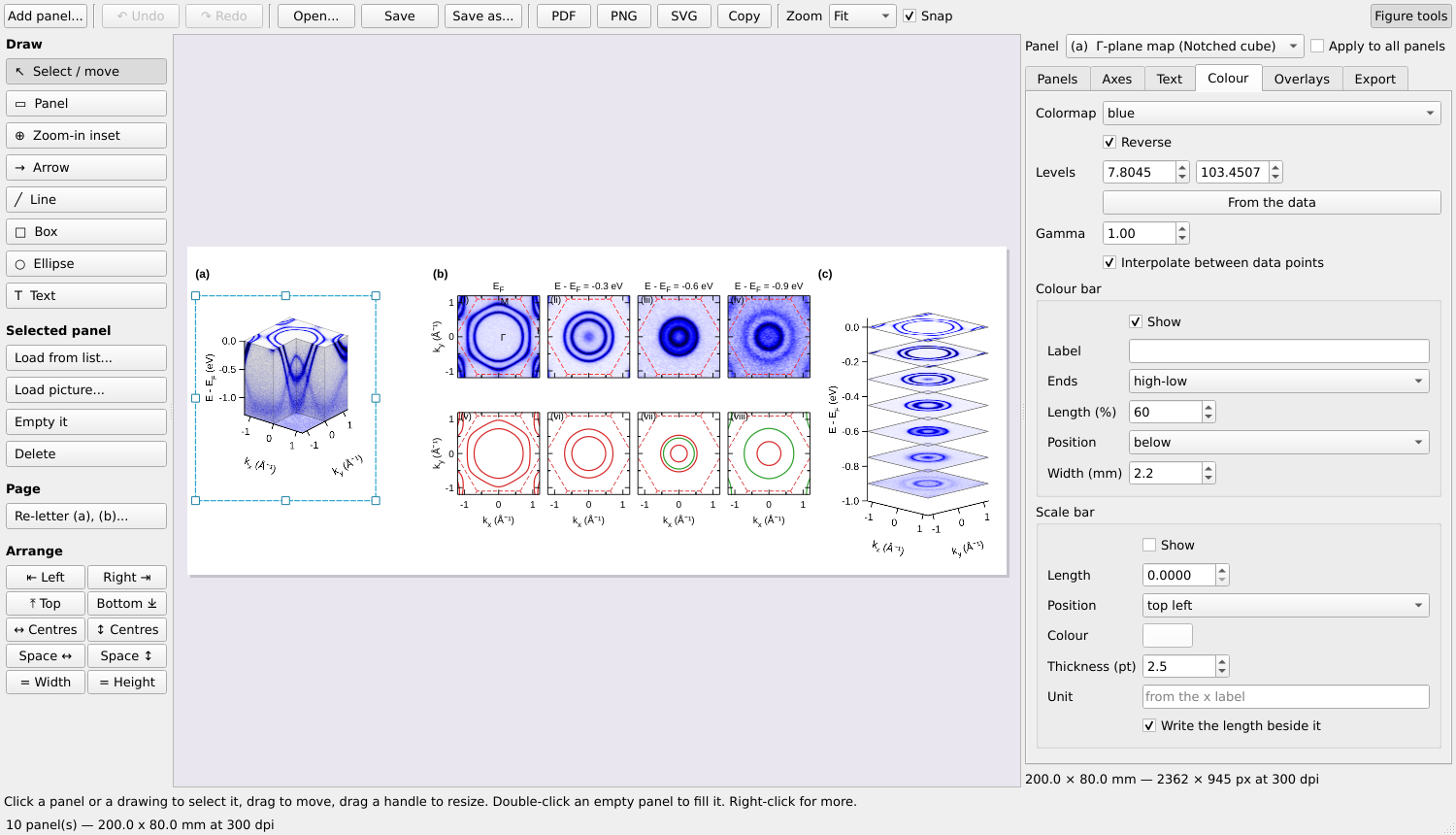
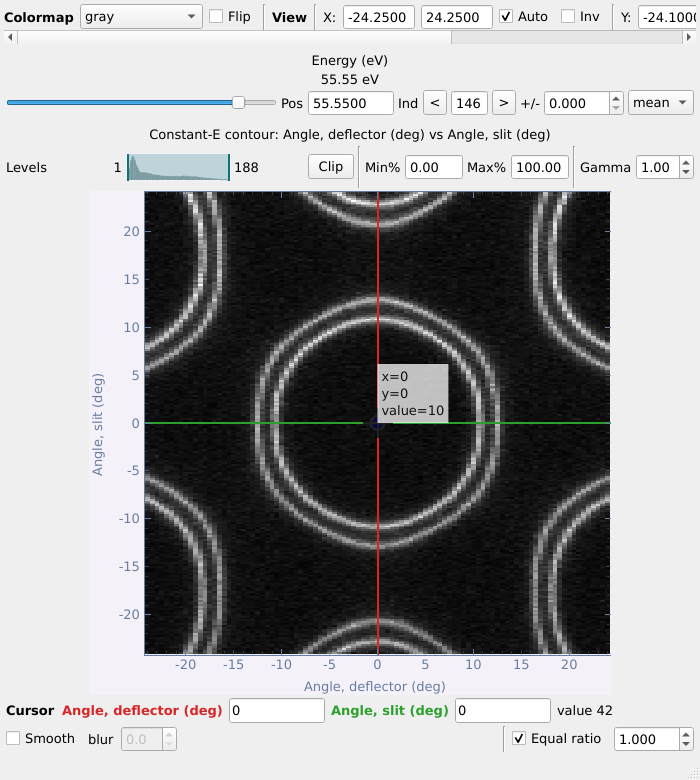
Example figure 1 in the figure composer (top); the main panel and a Fermi-surface map in momentum, in its viewer (bottom) -- also on the synthetic demo data.
Every step from the files to the finished figure is the program's own, and every step is plain Python that a script -- or an AI agent -- can run, without a screen:
| Step | In the program | In code |
|---|---|---|
| 1. Raw data | the beamline files, as the main panel lists them | arpes_viewer.loader.registry.load(path, entry) |
| 2. To momentum | the Γ-plane Fermi-surface map → k-map | arpes_viewer.tools.momentum.kspace.convert_map(...) |
| 3. The calculation | Calculated bands: a Wannier Hamiltonian; Z and the shift fitted on a cut | BandsDialog.open_file(...), .fit_alignment() |
| 4. Measured vs calculated | constant-energy maps over the calculated contours, coloured by orbital weight (b) | BandsDialog.series_panels(...) |
| 5. 3-D views | the notched cube (a), the stacked contours (c) | VolumeWindow(...).figure_panel() |
| 6. The figure | the figure composer: arranged, lettered, exported as PNG / PDF, saved as .afig with the data and the files it came from |
FigureWindow(...), .arrange(...), .write(...) |
devtools/figure_tests.py is exactly this script -- it writes the demo
files, reads them back, and builds this figure (and its companion, example
figure 2) in under a minute:
python devtools/figure_tests.py out_png/ out_afig/
In the step 3 fit it recovers what was built into the demo calculation (Z = 0.798 ± 0.001 and a shift of −49.8 ± 0.4 meV, against 0.8 and −50 meV).
An AI agent can drive it
Talk to your AI app (the Claude desktop app, Claude Code, any agent that can read and write files) in plain words -- "today I process the kz maps in this folder: align the Fermi levels, convert to momentum with Γ at 80 eV, draw the zone, and make a slice-series figure" -- and it drives the program on your screen, step by step, while you watch and can take over. Data stay on your computer.
- Start: press AI assistant... (top of the tool panel), choose the
data and results folders, tick what you want (step by step, a usage log,
a report, slides, hiding the sample's identity ...), and press Copy the
prompt and start; paste the prompt into your AI app. The window then
lists each step the agent runs, and Pause hands you the controls. The
agent reads
arpes_viewer/agent/API.md, the program's ~50 documented operations (L.fermi_edge,L.kz_to_k,L.bz_overlay,L.slice_series,L.figure_render...), instead of the source. - Other routes: an MCP app (
arpes-viewer-mcp; with the program started asarpes-viewer --agent-bridgeit calls the same operations), or a coding agent writing a script to keep, on the headless workspace and the Qt-free computations inarpes_viewer/tools/.
Starting and watching an agent from the AI assistant panel

- Open it. Press AI assistant... at the top of the main panel's tool column (above). The button is also the agent's status light, whether the window is open or not: grey not running, green running, yellow paused (you work by hand), red a failed step.
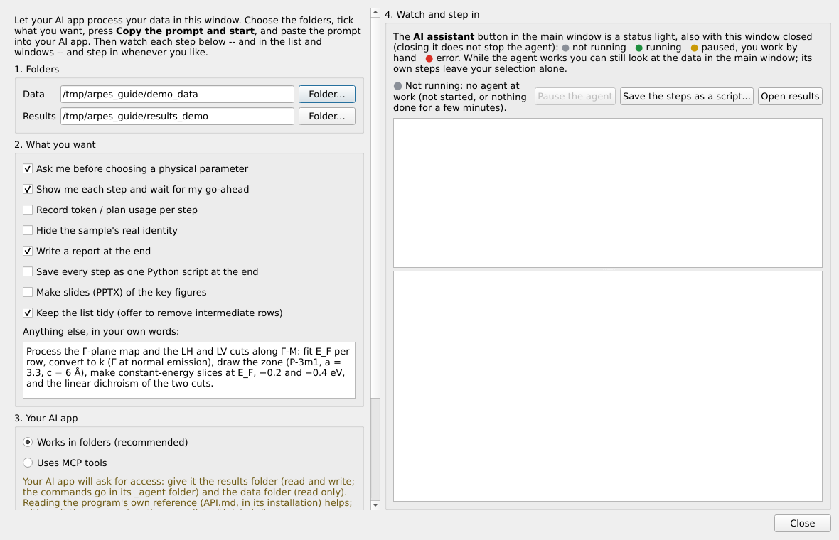
- Set it up (left column):
- 1. Folders: the data folder (read only for the agent) and a
results folder (everything it writes goes there; its commands go
in
<results>/_agent). - 2. What you want: ask before each physical parameter (Γ, an energy window, V0 ...), step by step with your go-ahead, a usage log, a report, slides, hiding the sample's identity, a tidy list -- and your request in your own words.
- 3. Your AI app: works in folders (the Claude desktop app, Claude Code, any agent that reads and writes files -- nothing to install) or uses MCP tools.
- 1. Folders: the data folder (read only for the agent) and a
results folder (everything it writes goes there; its commands go
in
- Start. Press Copy the prompt and start and paste the prompt
into your AI app. The prompt tells the agent where the folders are,
where the program's reference (
arpes_viewer/agent/API.md) is, and the working rules (fit E_F on raw data per row, report files left out, ask before going around an operation, keep the list tidy ...); Show the prompt shows it in full.
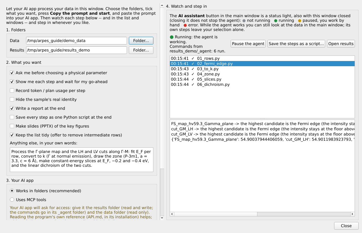
- Watch and step in (right column). Each step the agent runs appears in the list with ✓ or ✗ (red); click one to see what it printed -- here the Fermi-edge search and fit of a map. Its results appear as new rows in the main list (never overwriting anything), its pictures and figures in the results folder. Pause the agent holds its next commands while you work by hand (the light turns yellow); Resume lets them through. Closing the window does not stop the agent.
- Your screens stay yours. Windows the agent opens only to drive them (a conversion dialog, a temporary slice series) never appear; the ones it leaves open -- a finished figure, a viewer, a tool waiting for your input -- open on the screen of the main panel, not on the screen you are working on.
The step-by-step guide is agentic/README.md, with
requests to copy in agentic/PROMPTS.md; a real session
by Sonnet 5.5 is in Reports/.
As with any analysis, check what an agent produced before you publish it.
Bug reports
The program saves what went wrong by itself, in
error_logs/errors_<date>_<time>.txt in its folder (in ~/.arpes_viewer/
when installed with pip), and keeps running. With a bug report on
GitHub Issues,
upload that file (drag it into the text box) or paste its text --
the main panel's foot has Copy the newest error log and Open the
error logs -- and give the version number, shown in the main window's
title bar.
Documentation
- User guide, with screenshots: English · 中文 · Français; as PDF: English · 中文 · Français.
- AI agents: start with the beginner's guide
agentic/README.md-- connecting an agent step by step, runnable examples and requests to copy; then the MCP server (user guide, Part 7) and the file-based agentic workflow. - What changed, and why: CHANGELOG.md.
- Technical references, beside the code they describe -- the formulas,
the file layouts, the assumptions and the tests behind each step:
- Reading data -- every facility's files, the data kinds, adding a beamline, the assumptions the formats force;
- The windows -- the main panel, the viewers, autosave and recovery, long operations;
- Analysis -- what each tool does and what it assumes;
- Momentum conversion -- k conversion, k_z maps;
- Spectra -- core levels, curves, curve fits, spin;
- Processing -- de-gridding, cut arithmetic;
- Figures, export and the experiment log;
- For developers -- the layout of the code, and the
tests (
python -m pytest).
Terms of use, citation and licence
Terms of use. This program is for non-commercial use only (academic research and teaching); any commercial use is not permitted. New and updated loaders cover data from public large-scale facilities (synchrotrons and similar user facilities), formats of individual laboratories' own set-ups can be added by the user him/herself. If you use this program for a paper on ARPES experiments, please cite it in its references: Ding Pei, ARPES viewer, Zenodo, https://doi.org/10.5281/zenodo.23771647 (GitHub's Cite this repository gives the reference in other formats). If you write a paper related to AI that uses this program or its code, please discuss it with the author by e-mail first. For collaborations, or questions about the details, contact ding.pei@synchrotron-soleil.fr.
Licence and authorship. Copyright (c) 2026 Ding Pei. Licensed under the PolyForm Noncommercial License 1.0.0; see also NOTICE. This is the author's personal work, developed from the author's own earlier code; no institution funded it. Some of its ideas were inspired by the ARPES data-processing programs of the author's former group, the Chen Group at the University of Oxford. The requirements, design decisions, trade-offs, physics, the testing on real experimental data and the feedback from it (drawing on Phys. Rev. B 103, 245121 (2021) and Phys. Rev. B 95, 125126 (2017)), and the review and acceptance of every change are Ding Pei's; the implementation was assisted by Claude (Anthropic), credited as co-author in the commits.
1 maintainer

Metadata
1 maintainer
Release files for arpes-viewer 1.3.3
For a detailed explanation of source distributions (sdists) and built distributions (wheels), please see the package formats documentation.
Source distribution (sdist)
| File | Size | Uploaded | Provenance | Actions |
|---|---|---|---|---|
| arpes_viewer-1.3.3.tar.gz | 1.1 MB | With provenance | Details for arpes_viewer-1.3.3.tar.gz |
Built distribution (wheel)
| File | Interpreter | ABI | Platform | Actions Reset |
|---|---|---|---|---|
| arpes_viewer-1.3.3-py3-none-any.whl | Python 3 | none | any | Details for arpes_viewer-1.3.3-py3-none-any.whl |
Total release size: 2.3 MB
Release files / arpes_viewer-1.3.3.tar.gz
| Download URL | arpes_viewer-1.3.3.tar.gz |
|---|---|
| Size | 1.1 MB |
| Tags | Source |
|
SHA-256 checksum How to use checksums |
fc202d72df9882712d5c5888ce84cfedd0a9302842d51ffc273b7f10ea70c4de
|
|
BLAKE2b-256 checksum How to use checksums |
39629a61d2af637d411688be76dfd8641fb4972ad716bcbbfab051fb4234b30b
|
| Upload date | |
|
Uploaded using Trusted Publishing? What is trusted publishing? |
Yes |
| Uploaded via |
twine/7.0.0 CPython/3.13.16
|
Provenance
Provenance describes where a file came from. On PyPI, provenance is shared via attestations, which provide a verifiable record of the build or publishing details. View details, limitations and caveats.


PyPI Publish Attestation
PyPI verified that this artifact, at this checksum, originated from the publisher listed below.
Signed by GitHub Actions, verified by PyPI on Nov 10, 2026.
Transparency logRelease files / arpes_viewer-1.3.3-py3-none-any.whl
| Download URL | arpes_viewer-1.3.3-py3-none-any.whl |
|---|---|
| Size | 1.2 MB |
| Tags | Python 3 |
|
SHA-256 checksum How to use checksums |
306cb5c7581e79346ad6121bec94dcb8cc16427675340a07023c429b5967e9d9
|
|
BLAKE2b-256 checksum How to use checksums |
be3386c22ef7bca3c325c1ccbc387ac93e7f230a00d456cc2389c1ca9b96b8e2
|
| Upload date | |
|
Uploaded using Trusted Publishing? What is trusted publishing? |
Yes |
| Uploaded via |
twine/7.0.0 CPython/3.13.16
|
Provenance
Provenance describes where a file came from. On PyPI, provenance is shared via attestations, which provide a verifiable record of the build or publishing details. View details, limitations and caveats.
PyPI Publish Attestation
PyPI verified that this artifact, at this checksum, originated from the publisher listed below.
Signed by GitHub Actions, verified by PyPI on Nov 10, 2026.
Transparency logSecurity for arpes-viewer 1.3.3
Provenance
Provenance describes where a file came from. On PyPI, provenance is shared via attestations, which provide a verifiable record of the build or publishing details. View details, limitations and caveats.
Full provenance
Both files in this release have been uploaded with provenance metadata.
Attestation for arpes_viewer-1.3.3.tar.gz
PyPI Publish Attestation
PyPI verified that this artifact, at this checksum, originated from the publisher listed below.
Signed by GitHub Actions, verified by PyPI on Nov 10, 2026.
Transparency logA note on package security
PyPI is a repository for distributing packages, not a service for auditing them. While third-party security researchers and our staff do their best to detect and remove malicious packages, PyPI cannot guarantee the quality, security or suitability of any given package.
To learn more about protecting yourself from malicious actors, visit our package security documentation.














