A 3D monte carlo simulation of Atmospheric Radiative Transfer

Project description
AtmoRad
A vectorized Monte Carlo simulation of atmospheric radiative transfer.


| 2D Surface absorption map | Sample photon paths |
|---|---|
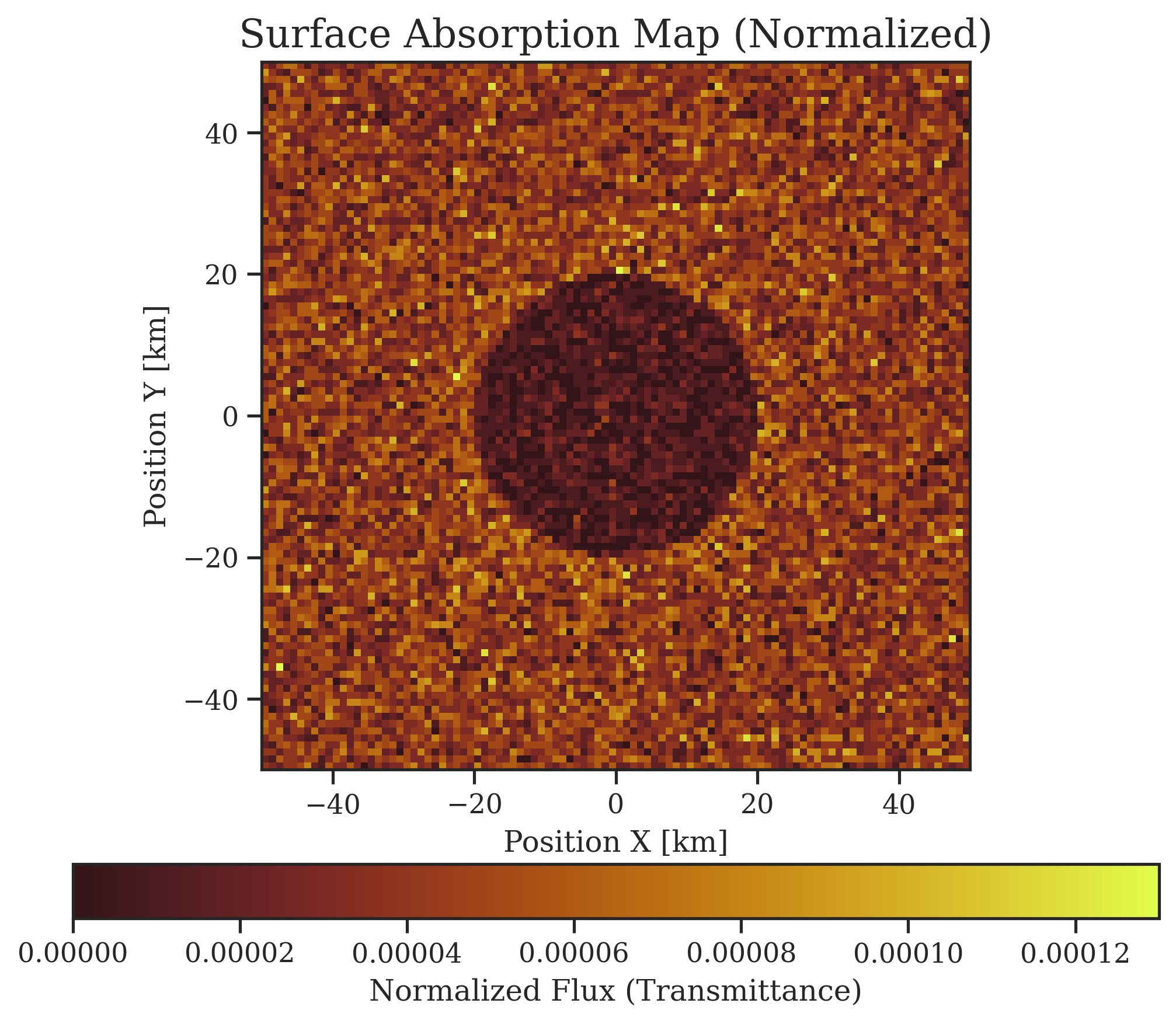 |
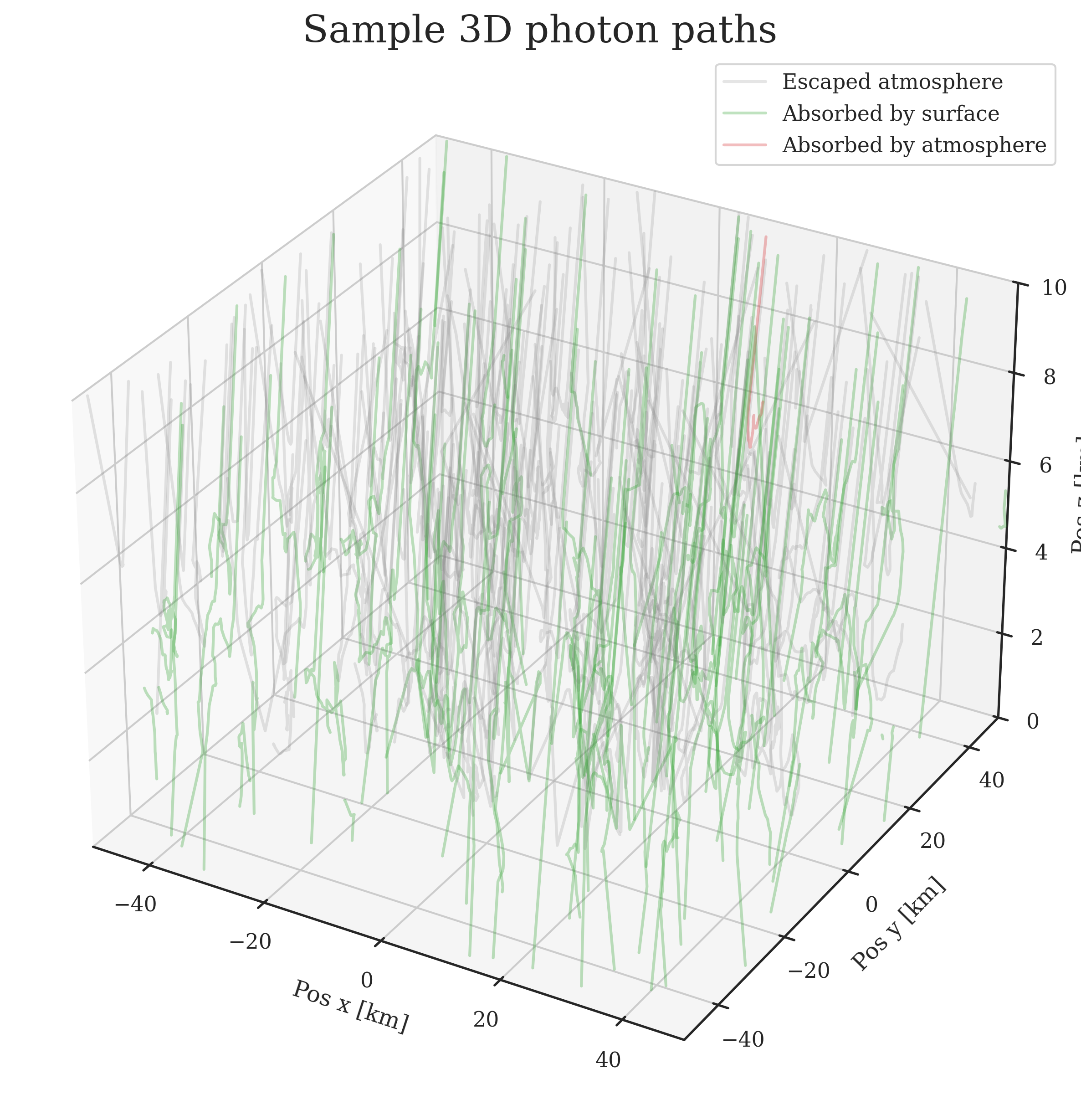 |
| Vertical flux profile | Vertical absorption profile |
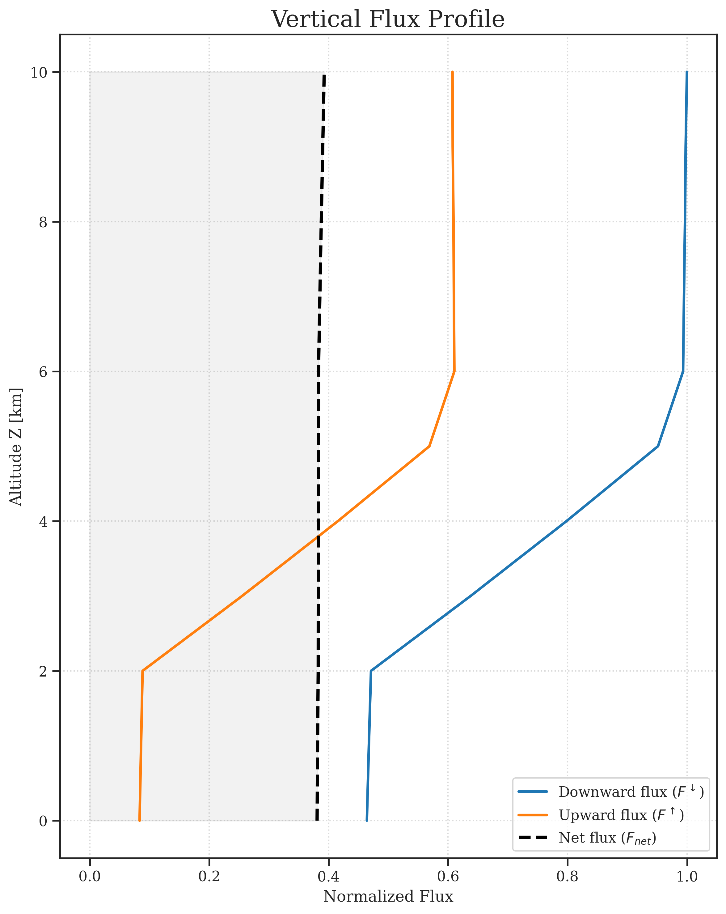 |
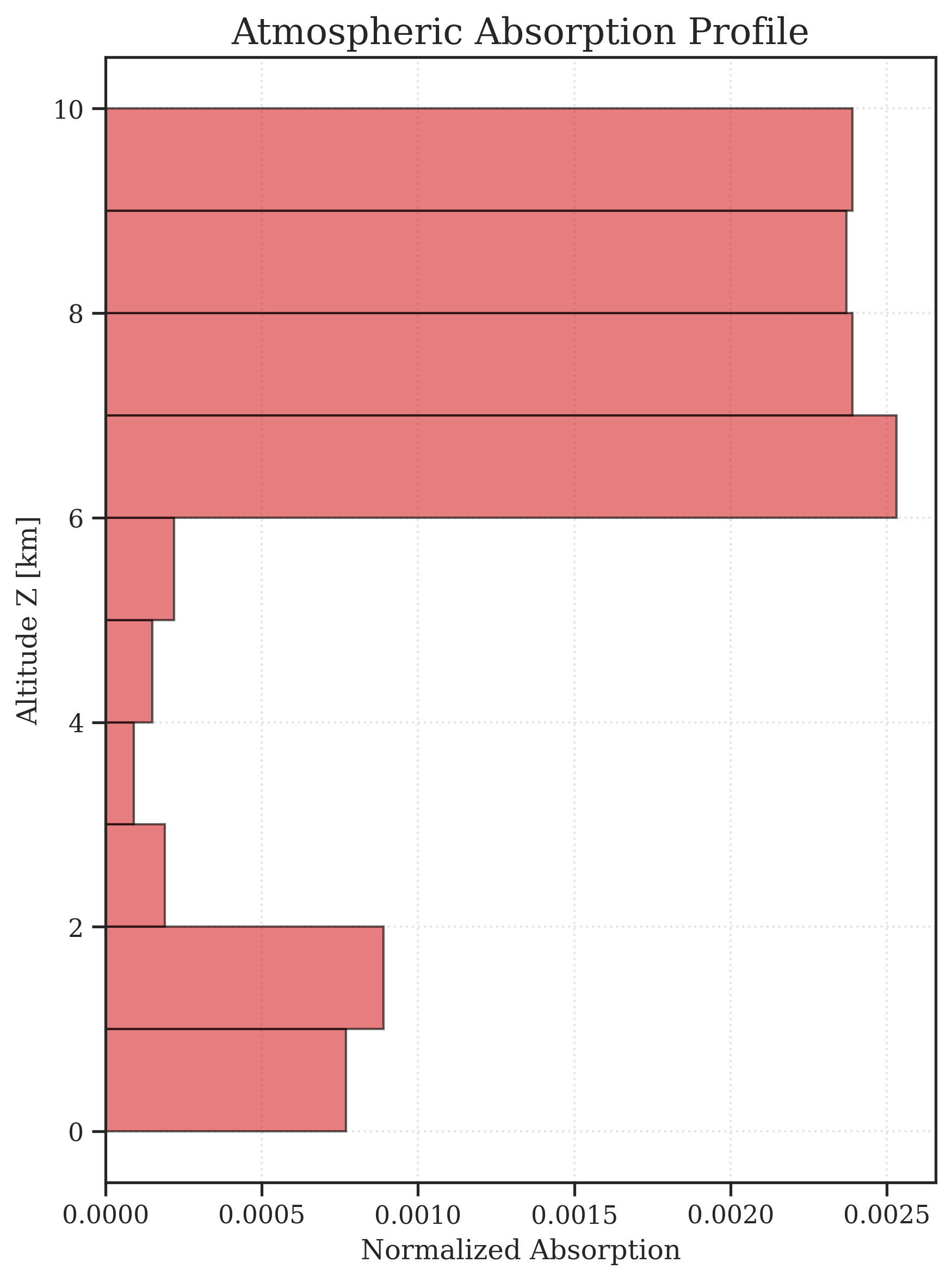 |
Overview
This project simulates the propagation of light through a plane-parallel atmosphere over a horizontally mixed surface and its interactions with the ground boundary. Developed as a student project to explore computational physics and software engineering, it uses numpy to simulate photons simultaneously in large batches via multiprocessing, and generates visualizations using matplotlib and seaborn.
Installation
Using uv (Recommended):
uv tool install atmorad-py
Using pip:
pip install atmorad-py
Quickstart
Initialize a default configuration file in your current directory:
atmorad --init
Run the simulation:
atmorad simulation.toml
Check the results/ directory for generated simulation artifacts and plots.
Physical Model
- Analog Monte Carlo Approach: Light is simulated using discrete photon packets. Final flux is calculated as a fraction of the total detected packets.
- Plane-parallel approximation: The atmosphere consists of horizontally uniform layers.
- Multi-material atmospheric layers: Layers can consist of multiple atmospheric materials simultaneously. A photon is assigned a material randomly when it is initialized and again when it crosses into a new layer. Each material has its own extinction coefficient, SSA, and phase function.
- Custom Phase Functions: Henyey-Greenstein and Rayleigh phase functions are built-in, but any custom user-defined function can be constructed using the
Scatteringclass. - Surface Reflections: The surface consists of materials, each with its own albedo, a predefined BRDF reflection model (
Lambertian,Specular), and aProceduralMapthat outputs material IDs based on spatial coordinates. - Photon Properties: Light is treated as monochromatic, non-polarized particles. During the simulation they can be scattered, reflected, or absorbed.
- Incident Irradiance & Adjacency Effect: Custom detectors allow measuring downward/upward incident flux at any arbitrary altitude, which is helpful for visualizing the adjacency effect.
Customization
You can define your own surface maps, surface reflection algorithms, and scattering phase functions using decorators as shown below:
import numpy as np
import atmorad
from atmorad import SurfaceReflection, register_reflection, orientation
from atmorad import Scattering, register_scattering
from atmorad import BaseSurfaceMap, register_surface_map
from atmorad.constants import X, Y

# 1. Registering a custom surface map
@register_surface_map("custom-stripe-y", ["material_name_a", "material_name_b"])
class StripeYMap(BaseSurfaceMap):
    # Specify arbitrary custom parameters
    def __init__(self, stripe_width_km: float):
        self.width = stripe_width_km

    def get_material_ids(self, pos: np.ndarray) -> np.ndarray:
        # Maps 2D photon coordinates to integer indices (0 for material_name_a, 1 for material_name_b)
        # Your custom geometry logic here
        grid_x = np.mod(pos[X], self.width)
        return np.where(grid_x < (self.width / 2.0), 0, 1)

# 2. Registering a custom surface reflection
@register_reflection("custom-reflection")
class CustomReflection(SurfaceReflection):
    def __init__(self, param_1, param_2):
        self.param_1 = param_1
        self.param_2 = param_2

    def reflect(self, direction, rand_1, rand_2):
        cos_theta = np.sqrt(rand_1)
        sin_theta = np.sqrt(1.0 - rand_1)
        phi = rand_2 * 2 * np.pi
        cos_phi, sin_phi = np.cos(phi), np.sin(phi)
        return orientation(cos_theta, sin_theta, cos_phi, sin_phi)

# 3. Registering a custom scattering phase function
@register_scattering("custom-scattering")
class CustomScattering(Scattering):
    def __init__(self, g, resolution=1000):
        self.assymetry_factor = g
        cos_grid = np.linspace(-1, 1, resolution)
        pdf = (1 - g**2) / (2 * (1 + g**2 - 2 * g * cos_grid) ** 1.5)
        super().__init__(pdf_array=pdf, resolution=resolution)

if __name__ == "__main__":
    # 4. Running the simulation from config which uses your custom names
    results = atmorad.run("simulation.toml")
    # Figures and metadata are saved automatically
    # You can also process results on your own
In simulation.toml you can specify your defined scatterings, reflections and surface maps:
[atmosphere_materials.custom-atm-material]
ssa = 0.9
scattering = {type = "custom-scattering", g=0.8}

[surface_materials.custom-surf-material-a]
albedo = 0.5
reflection = {type = "custom-reflection", param_1=2, param_2=1.3}

[surface_materials.custom-surf-material-b]
albedo = 0.1
reflection = {type = "lambertian"}
Then you can use your defined materials for atmospheric layers and the surface:
[[layer]]
thickness_km = 2
materials = [{type = "custom-atm-material", weight = 1.0}]

# ...

[surface]
name = "custom-stripe-y"
stripe_width_km = 5.0 # include parameters required for this map type
material_name_a = "custom-surf-material-a"
material_name_b = "custom-surf-material-b"
Loading Results
Once a simulation finishes, you can easily load the results and the exact configuration used into a Python environment (like a Jupyter Notebook) for analysis:
import atmorad
import matplotlib.pyplot as plt

# 1. Loading the completed simulation
config, results = atmorad.load("results/demo001")

# 2. Accessing your physical data as NumPy arrays
map_2d = results.detectors["boundary_flux"].surface_absorption_map_2d

# 3. Analysis or plotting
plt.imshow(map_2d)
plt.title(f"Flux Map for {config.metadata.experiment_name}")
plt.show()
Project Structure
engine/: Divides photons into batches and runs the simulation.physics/: Contains a rotation function, scattering phase functions, reflection functions.environment/: Keeps track of the environment. ContainsScene,AtmosphereandSurfaceclasses.detectors/: Provides functionality for tracking photons during the simulation and generates results.output/: Handles results and figure generation.config/andbuilder.py: Parses.tomlconfiguration file and generates simulation context.cli.py: Provides CLI foratmorad.
References and Literature
- (in Polish) Script for Lecture about Radiative Processes in the Atmosphere, Prof. K. Markowicz, Faculty of Physics, University of Warsaw, 2013.
Acknowledgments
- This project was inspired by the lectures on Radiative Processes in the Atmosphere by Prof. K. Markowicz, Faculty of Physics, University of Warsaw.
- Large Language Models were used for code debugging and learning best Python practices (e.g.
dataclasses,__init__.pyimport interfaces, class responsibilities, config parsing).
Contributing
Feel free to open an Issue or submit a Pull Request if you'd like to contribute or report a bug.
Release history Release notifications | RSS feed


Download files
Download the file for your platform. If you're not sure which to choose, learn more about installing packages.
Source Distribution
Built Distribution
Filter files by name, interpreter, ABI, and platform.
If you're not sure about the file name format, learn more about wheel file names.
Copy a direct link to the current filters
File details
Details for the file atmorad_py-0.2.0.tar.gz.
File metadata
- Download URL: atmorad_py-0.2.0.tar.gz
- Upload date:
- Size: 131.4 kB
- Tags: Source
- Uploaded using Trusted Publishing? No
- Uploaded via: uv/0.11.3 {"installer":{"name":"uv","version":"0.11.3","subcommand":["publish"]},"python":null,"implementation":{"name":null,"version":null},"distro":{"name":"Ubuntu","version":"24.04","id":"noble","libc":null},"system":{"name":null,"release":null},"cpu":null,"openssl_version":null,"setuptools_version":null,"rustc_version":null,"ci":null}
File hashes
| Algorithm | Hash digest | |
|---|---|---|
| SHA256 |
c69fb9ffe93934c4ea85f388ad6cf77a9e8cec303f7b815d3162015771741645
|
|
| MD5 |
26ba9dc144e54303d6b89c79f70f4c8d
|
|
| BLAKE2b-256 |
18f18aecf620ff84fbcad07e18892a2c291b53041cebbd05a7f0230ab89aa1e8
|
File details
Details for the file atmorad_py-0.2.0-py3-none-any.whl.
File metadata
- Download URL: atmorad_py-0.2.0-py3-none-any.whl
- Upload date:
- Size: 42.9 kB
- Tags: Python 3
- Uploaded using Trusted Publishing? No
- Uploaded via: uv/0.11.3 {"installer":{"name":"uv","version":"0.11.3","subcommand":["publish"]},"python":null,"implementation":{"name":null,"version":null},"distro":{"name":"Ubuntu","version":"24.04","id":"noble","libc":null},"system":{"name":null,"release":null},"cpu":null,"openssl_version":null,"setuptools_version":null,"rustc_version":null,"ci":null}
File hashes
| Algorithm | Hash digest | |
|---|---|---|
| SHA256 |
ae18d24f8e168b682cfa87f96757a1dd0eba91d8c3bb47f02697305f72216fac
|
|
| MD5 |
208ff1db3f6aeaec918f0e05bcd6a769
|
|
| BLAKE2b-256 |
ea15802af639fb9f13063174d6f169fef09ac20eedc2db73cb9b4d6e96999fd6
|


