
auto-optimal-control
Express an optimal control problem symbolically and get every function the indirect (costate) method needs to solve it as a two-point boundary value problem: the Hamiltonian, the optimal control law, switching functions for bang-bang controls, the state–costate dynamics and the boundary-condition residuals.
Integration runs on fast-numerical-integration (FNI), which this package depends on from PyPI.
Status: pre-alpha. Symbolic problem definition, Pontryagin derivation, generated and compiled C kernels, and arc-by-arc propagation of extremals with the state transition matrix are in place.
The core operation is the forward map from an initial costate to an
extremal: pick lambda(t_0) and get the optimal trajectory, its controls,
its cost, its switch times, its boundary residuals and, if you want them,
exact sensitivities. The package doesn't decide how lambda(t_0) is chosen.
Shooting, multiple shooting, continuation, or a learned sampler that proposes
costates can all be built on top of the same calls. One such layer ships with
the package, optionally: auto_optimal_control.shooting, a single-shooting
system with exact Jacobians and a solver.
Installation
pip install "auto-optimal-control[shooting]" # or: uv add "auto-optimal-control[shooting]"
The shooting extra adds SciPy, which SingleShooting and
MultiArcShooting use for their root finders. Leave it out if you only need
the derivation and the compiled kernels. The kernels are compiled when you
first build them, so you need a C compiler (gcc or clang). The
fast-numerical-integration
dependency installs as a pre-built wheel on Linux x86_64 and macOS arm64.
To work on the package itself:
git clone https://github.com/idm23/auto-optimal-control
cd auto-optimal-control
uv sync
uv run pytest                 # add --runslow for the literature benchmarks
Example: minimum-time double integrator
import sympy as sp
from auto_optimal_control.problem import Box, OptimalControlProblem
from auto_optimal_control.pontryagin import derive

t, x, v, u = sp.symbols("t x v u", real=True)
problem = OptimalControlProblem(
    time=t, states=[x, v], controls=[u],
    dynamics=[v, u], running_cost=1,                # minimum time
    initial_state=[1, 0], final_state={x: 0, v: 0},
    control_sets=[Box(u, -1, 1)])                   # |u| <= 1

pmp = derive(problem)
pmp.hamiltonian                  # Piecewise: 1 + lam_x v - |lam_v|
pmp.control_law[u]               # Piecewise((1, lam_v < 0), (-1, True))
pmp.switching_functions[0].expr  # lam_v
pmp.dynamics                     # (v, u*, 0, -lam_x) for z = [x, v, lam_x, lam_v]
pmp.boundary.residuals           # x(t_0) - 1, v(t_0), x(t_f), v(t_f), transversality, H(t_f)
pmp.boundary.unknowns            # x(t_0), v(t_0), lam_x(t_0), lam_v(t_0), nu_0, nu_1, t_f
Compile it and evaluate extremals from any initial costate:
from auto_optimal_control.build import build_kernels

k = build_kernels(pmp)           # generate C, compile (cached), load
r = k.propagate(0.0, k.z0([1, 1]), 2.0, cost=True, stm=True)
r["switch_times"]                # [1.0]: u switches from -1 to +1
r["z"]                           # [x, v, lam_x, lam_v] at t = 2: x = v = 0
r["cost"]                        # 2.0 (minimum time)
r["stm"]                         # dz(2)/dz(0), including the jump at the switch
k.residual(k.z0([1, 1]), r["z"], r["z"][2:], 2.0)   # ~0 (nu = lam(t_f))
Using the compiled kernels
build_kernels(pmp) prints the necessary conditions as plain C (see
codegen.py for the function list), wraps them for
fast-numerical-integration's
GIL-free C API, compiles both and returns a Kernels object. Builds are
cached by a hash of the generated code and the toolchain. The first build
takes about 10 s and later ones load instantly, across processes too. The
cache is in ~/.cache/auto-optimal-control, or $AUTO_OPTIMAL_CONTROL_CACHE
if set. Building needs a C compiler.
The forward map (from an initial costate to an extremal):
| Call | Returns |
|---|---|
k.propagate(t0, z0, t1, params, cost=, stm=, param_sensitivity=) |
final z, switch times, cost J = int L, and optionally Phi = dz(t1)/dz(t0), dz(t1)/dp and dz(t1)/dt1 |
k.propagate_batch(t0, Z0, t1, params, ..., n_threads=) |
the same for many rows at once, in parallel threads without the GIL; each row is bit-identical to propagate |
k.trajectory(t0, z0, t1, params, n_points=) |
sampled t, z, controls u and H, for plots and diagnostics |
k.z0(lam0, params) |
[x0, lam0] from the problem's fixed initial state |
Propagation runs arc by arc, as one FNI hybrid integration
(fni_integrate_hybrid, FNI >= 0.3). Each switching function is a guard,
located to round-off, and its reset map applies the saltation-matrix jump to
the STM and flips the arc. No integration step straddles the jump in the
control, and the step size carries across switches.
Pointwise kernels: rhs, rhs_arc, jacobian (dF/dz), dfdp,
control, hamiltonian, cost_rate, switching, switching_gradient,
residual, residual_jacobian (with respect to z0, zf, nu, tf, p)
and stm_jump.
FNI objects: k.Dynamics(params) and k.ArcDynamics(params, arc, stm=)
are native OdeSystems, and k.switching_events(params) gives native
EventFunctions. They work with FNI's solve_ivp, integrate and
integrate_batch, and their params can be changed between solves without
recompiling.
Plain C: k.write_c(directory) writes the header and source on their
own; they depend only on <math.h>.
Speed (planar low-thrust example, 10 states, 3 switches, DOP853 at
rtol=1e-10):
| time per extremal | |
|---|---|
NumPy reference (NumericSystem + FNI solve_ivp) |
67 ms |
k.propagate |
0.05 ms |
k.propagate(..., stm=True) (110 states) |
0.28 ms |
k.propagate_batch, 1000 rows, 1 thread / 16 threads |
36 µs / 11 µs |
auto_optimal_control.numeric.NumericSystem is still there as a
pure-Python reference (lambdified with SymPy); the kernel tests compare
against it.
Single shooting (optional)
auto_optimal_control.shooting turns the forward map into a square system
R(v) = 0. Nothing else in the package imports it. The unknowns v are
the free initial states, lam0, the terminal multipliers nu, and t_f
when it is free. The Jacobian is exact: the generated boundary Jacobians
chained with the STM, with the jumps at switches included.
from auto_optimal_control.shooting import SingleShooting, continuation

shoot = SingleShooting(k, params)              # x0 defaults to the problem's
v = shoot.guess_multipliers(lam0, tf=2.0)      # least-squares nu for this lam0
R, dR = shoot.residual_jacobian(v)             # NumPy only: drive it with anything
sol = shoot.solve(v)                           # MINPACK hybr / lm, needs SciPy
sol.success, sol.lam0, sol.tf, sol.z0
multistart(sample, n_tries)solves from random guesses until one converges.continuation(solve_at, start, values, v0)follows a homotopy parameter. It halves the step whenever a solve fails.trajectory(v)samples the extremal atv.
solve needs SciPy: pip install auto-optimal-control[shooting]. The
residual and Jacobian need only NumPy, so a sampler or any other solver can
use them directly.
Defining a problem
OptimalControlProblem is in Bolza form:
minimize    phi(t_f, x(t_f)) + integral L(t, x, u) dt
subject to  x' = f(t, x, u),   x_i(t_0) fixed (or free),   psi(t_f, x(t_f)) = 0,   u in U
- Parameters (
params=[...]) stay symbolic, so one derivation (and later one compiled kernel) serves a whole continuation sweep. Their order is the order of FNI's runtime parameter vector. - Final time is free by default; pass
final_time=to fix it. - Control sets: controls are unconstrained unless placed in a set.
Box(u, lower, upper): a Hamiltonian linear inugives bang-bang control with a switching function; a convex quadratic one gives a saturated (clipped) control.UnitVector([u1, u2, ...]): a direction such as a thrust direction or a heading. The optimum is-b/||b||(the primer vector for thrust).
- Declare positive quantities (masses, thrust, speeds) with
positive=True. The derivation relies on it to simplify norms and to prove convexity.
Path constraints
State limits g(t, x, p) <= 0, such as joint limits, a keep-out radius or a
speed limit, are declared on the problem:
from auto_optimal_control.problem import PathConstraint

OptimalControlProblem(..., params=[ell, rho],
                      path_constraints=[PathConstraint(x - ell, "x_max", penalty=rho)])
- Order.
derivedifferentiatesgalong the dynamics until a control appears. The number of derivatives is the constraint's order (pmp.path_constraints[i].order). A box on a control is order 0. A position limit on a double integrator is order 2. Order 3 or more warns: optimal solutions that ride such a limit generally chatter, with infinitely many touch points. A limit no control can reach raises an error. - Penalty. With
penalty=w(a parameter),w/2 max(0, g)^2is added to the running cost. Raisewby continuation (shooting.parameter_continuation) and the solution approaches the constrained one from below. Each constraint has its own flag in the arc (N_MODES = N_SWITCHING + N_CONSTRAINTSflags). Crossings ofg = 0are located as events and switch the penalty on and off. The dynamics are continuous there, so the STM has no jump. Without a penalty, a constraint only monitors: crossings are reported and the extremal is unchanged. - Termination.
propagate(..., terminate=True)(or indices or names) stops at the first violation with status-4, andtis its time. It stops att0if the start already violates.propagate_batch,trajectoryandSingleShooting(terminate=...)take it too, and shooting then raisesShootingError. This is the death penalty for gradient-free search: any violating extremal is rejected outright. For a safety margin, put it ingas a parameter. - Results.
propagatereturnsconstraint_times/constraint_index,trajectoryreturnsgalong the extremal, andShootingSolutionhasmax_violation.
Detecting crossings inside a step. An integrator that checks g only at
the ends of its steps misses a violation that starts and ends within one
step. Away from the limit the solution is smooth and steps are long, so this
happens easily. A missed crossing makes the residual run and the STM run
disagree about the dynamics, and Newton stalls. Two mechanisms prevent it:
 g   +           ╭──●──╮                ġ = 0 at the peak is an event: FNI splits
   0 ──────────┼─┼─────┼─┼──────        the step there, and g is monotone on each
     ●━━━━━━━━━╯         ╰━━━━━━●        side, so each side crosses zero at most once
     t_a        rise │ fall      t_b
- Every constraint gets a second event on
dg/dt, the peaks and troughs ofg. It has no reset map. FNI (0.4+) splits a step at every root it finds, so between consecutive peaks and troughs,gcrosses zero at most once and the crossing is found. - A peak and a trough can still fall in the same step. With the penalty off,
the flow overshoots, then turns back. For that case, kernels with path
constraints also use FNI's interior sign tests, at
n_interiorpoints per step (default 4).n_interior=0turns them off. They cost 3 extra RHS evaluations per step with DOP853.
The reset map sets each constraint's flag from the sign of dg/dt at the
crossing, so the flag always matches the side the flow moves to.
Exact boundary arcs and touch points
The penalty solution only approaches the constrained optimum.
MultiArcShooting solves for it exactly, given the sequence of constrained
arcs:
from auto_optimal_control.shooting import MultiArcShooting

# The penalty solution at rho supplies the structure's junction times and multipliers.
shoot, v0 = MultiArcShooting.from_penalty(k, [ell, 0.0], [("boundary", "x_max")],
                                          penalty_solution, [ell, rho])
sol = shoot.solve(v0)
shoot.unpack_arcs(sol.v)        # [(t_entry, t_exit, pi)]
shoot.cost(sol.v), shoot.diagnostics(sol.v), shoot.trajectory(sol.v)
-
Boundary arc
("boundary", c), for order 1 or 2. Along it the control keepsg^(q) = 0.derivefinds it, together with the multipliermuofH + mu g^(q), fromg^(q) = 0anddH/du + mu dg^(q)/du = 0. The costates jump by-dN/dx^T piat the entry, whereN = (g, ..., g^(q-1)) = 0, and are continuous at the exit.His continuous at both junctions (indirect adjoining; Bryson, Denham & Dreyfus 1963; Maurer 1977). Unknowns: entry, exit andpi. -
Touch point
("touch", c), for order 2:g = g' = 0at the contact, withlambda+ = lambda- - nu dg/dx. Unknowns: the time andnu. -
Exact Jacobian. The STM is chained across arcs, with the derivatives of each jump and of each junction time.
-
Checks.
diagnosticsreports violations on the free arcs (a wrong structure shows up there),nu(it must be ≥ 0),pi, and the range ofmuand of the controls on each boundary arc. -
Seeding from a penalty solution.
from_penaltytakes junction times from a penalty solution's crossings. A penalized boundary arc may dip back below the limit, so each arc spans its first to last crossing. It fitspiby integrating the boundary arc back from the exit. -
Bounded controls.
Boxcontrols keep their law on the free arcs: clipped whereHis quadratic in them, bang-bang where it is linear, with every switch located as in single shooting. On a boundary arc the control is the one that rides the limit, and it must stay inside its bounds there:diagnosticsreportsboundary_bound_violation, and it counts towardmax_violation. With bang-bang controlssolvedefaults to"lm". The control jumps at the junctions, soHcontinuity reads|S| = 0there, which stalls the Broyden updates of"hybr". -
Seeding a bang-bang problem. Its penalty solution is no use: the penalized optimum rides the limit on a singular arc. Smooth it instead. Add
eps u^2/2to the running cost, solve that with exact arcs (from a penalty solution as above), and lowerepsbycontinuation. The two problems have the same unknowns, so the last smoothedvseeds the bang-bang solve:def smoothed(eps, guess): return MultiArcShooting(k_smooth, [V, D, u_max, eps, 0.0], arcs).solve(guess) path = continuation(smoothed, 1.0, np.logspace(0, -4, 17), v_smooth) sol = MultiArcShooting(k_bang, [V, D, u_max], arcs).solve(path[-1][1].v)
velocity_limited_move (order 1, with and without a force limit),
bryson_denham (order 2, both regimes) and speed_limited_min_time
(bang-bang) are solved against their closed forms.
What derive produces
derive(problem) returns a PontryaginSystem:
| Attribute | Contents |
|---|---|
costates |
lam_<state>, one per state |
hamiltonian_full |
H = L + lam . f with the controls symbolic |
control_law |
u*(t, x, lam, p) minimizing H |
switching_functions |
SwitchingFunction(control, expr, lower, upper) per bang-bang control: u = upper where expr < 0 |
hamiltonian |
H at u*; constant along extremals when is_autonomous |
dynamics |
z' = F(t, z, p) for z = [x, lam]: x' = dH/dlam, lam' = -dH/dx |
running_cost |
L at u*, to accumulate the cost |
path_constraints |
StateConstraint(name, expr, order, derivatives, penalty) per path constraint |
penalty |
sum w/2 max(0, g)^2, included in hamiltonian, dynamics and running_cost |
path_constraints[c].boundary |
BoundaryArc(control, multiplier, dynamics, hamiltonian, running_cost, bounds) for exact arcs (orders 1 and 2), or None with the reason in unsupported |
boundary |
the boundary conditions: residuals, unknowns and the boundary symbols |
The boundary residuals are the fixed initial states (or lam_i(t_0) = 0 when
free), the terminal constraints psi, transversality
lam(t_f) = d(phi + nu . psi)/dx, and H(t_f) + d(phi + nu . psi)/dt = 0
when the final time is free. There are as many residuals as unknowns.
auto_optimal_control.examples has the problems the tests use: Zermelo's
navigation problem, minimum-time and minimum-energy double integrators
(unbounded and saturated), a terminal-cost LQ problem and a fuel-optimal
planar low-thrust transfer, the Bryson–Denham problem (an order-2 state
limit) and a velocity-limited move (an order-1 limit).
Tests
uv run pytest (about 30 s; it compiles every example from scratch) checks the following; uv run pytest --runslow (about 3 min) adds the benchmarks:
test_problem.py: problem validation.test_derivation.py: each example's Hamiltonian, control law, switching function, costate equations and boundary conditions against the textbook forms. On every example at random points,u*minimizesHover the admissible controls and the dynamics are Hamilton's equations ofH*.test_extremals.py: extremals of the NumPy reference, integrated with FNI from known optimal costates. They reproduce the analytic solutions and satisfy every derived boundary condition.test_kernels.py:- Every C kernel agrees with the NumPy reference at random points.
- Every derivative kernel agrees with finite differences.
- The plain C compiles under
-Wall -Wextra -Werror -pedantic. - The cache is reused.
- Native systems release the GIL.
test_propagation.py:- Switch times, costs and endpoints match the analytic answers.
- The STM and
dz/dpmatch finite differences of the forward map across switches. - Leaving out the jump gives the wrong STM.
- Batches equal single propagations, and threads agree with serial runs.
test_benchmarks.py(slow;--runslow): every literature benchmark above.test_visuals.py(slow; skipped without matplotlib): records each animated solve (cart-pole, Earth–Mars, Bryson–Denham), checks that its stages end where the benchmark does, and renders a small GIF and the stills.test_jacobian_chain.py: a bare Newton iteration built from the kernels converges quadratically, which shows the derivatives compose into an exact Jacobian, using the raw kernels rather than the shooting module.test_path_constraints.py: constraint order (1, 2 and 3 on a jerk chain, a planet radius, an unreachable limit). Monitor constraints leave the dynamics alone. Every run of one extremal sees the same crossings, and the STM matches finite differences across them. Bryson–Denham penalty continuation reaches both closed forms. Termination is checked inpropagate, batches,trajectoryand shooting.test_exact_arcs.py: boundary-arc derivation; the exact-arc kernels against finite differences;MultiArcShootingon order-1 and order-2 boundary arcs and a touch point, against closed forms (costates, junction times, jumps, cost), seeded from penalty solutions. The same with a clipped control (saturated, then a ramp onto the limit) and with a bang-bang one (full power, cruise, brake), seeded by smoothing continuation. Also its Jacobian against finite differences (across switches too), a wrong structure detected as a free-arc violation, the saturation guards, and validation.test_shooting.py:SingleShooting's unknown layout, its Jacobian against finite differences (including a free initial state), solves against closed forms, multistart and continuation.
Benchmarks against the literature
benchmarks/ solves nine canonical problems from scratch and compares each
indirect solution with a published value. It starts from random costate
guesses, uses continuation where needed, and for the cart-pole lifts
costates from a direct solution. Run them with
uv run python benchmarks/run.py; uv run pytest --runslow, which CI runs,
checks them too. They are solved with auto_optimal_control.shooting.
| Benchmark | Quantity | This package | Reference | Source |
|---|---|---|---|---|
| Brachistochrone (3 cases) | t_f |
matches to 1e-13 | closed-form cycloid | — |
Bryson–Denham, touch point (l = 0.2, ρ = 1e8) |
∫u²/2 |
2.2399263 | 2.24 | closed form (Bryson, Denham & Dreyfus 1963) |
Bryson–Denham, boundary arc (l = 0.1, ρ = 1e7) |
∫u²/2 |
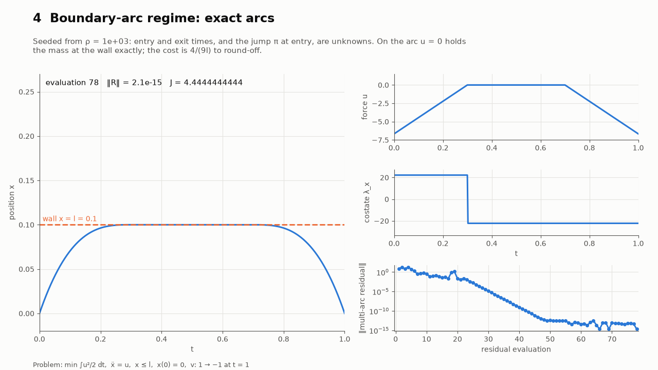
4.4430848 | 4.4444444 | closed form, 4/(9l) |
| Bryson–Denham, both regimes, exact arcs | ∫u²/2 |
matches to 1e-14 | closed form | — |
| Velocity-limited move (order 1, 3 cases), exact arcs | ∫u²/2 |
matches to 1e-14 | closed form, 4V²/(3t₁) |
— |
| Velocity-limited move with a force limit (2 cases), exact arcs | ∫u²/2 |
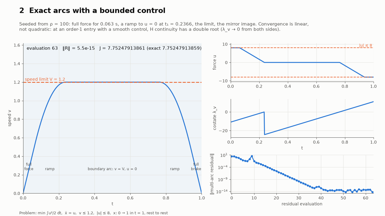
matches to 1e-12 | closed form (saturated, a ramp, the limit) | — |
| Minimum time with a speed limit (2 cases), bang-bang exact arcs | t_f |
matches to 1e-15 | closed form, D/V + V/u_max |
— |
| Maximum-radius orbit transfer | r(t_f) |
1.5252777 | 1.5252776 | Bryson & Ho (1975) pp. 66–69; value from YAPSS/IPOPT |
| Earth–Mars fuel-optimal rendezvous | m(t_f) |
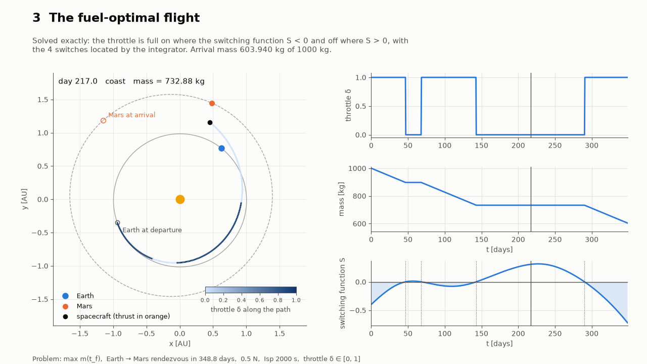
603.9402 kg | 603.935 kg | arXiv:2409.01490, Tables 1–2 |
| COPS robot arm, minimum time | t_f |
9.1409117 | 9.1409 | COPS #8 (Dolan, Moré & Munson); GAMS NOA, PROPT |
| Cart-pole swing-up (published extremal) | ∫u² |
58.807667 | 58.80819 | Kelly (2017) SIAM Review; value from the ASSET reproduction |
| Cart-pole swing-up (random search) | ∫u² |
57.944780 | — | this work; checked by an independent simulation |
Notes:
- The reference values come from direct (collocation) methods or smoothed controls, so agreement to 1e-6–1e-5 is what to expect. The indirect solutions here locate switches exactly. On Earth–Mars, the exact bang-bang solution keeps 0.005 kg more mass than the smoothed one (ρ = 1e-5), which is the expected sign. It has four switches, at 46.6, 68.0, 142.7 and 290.3 days.
- Robot arm: pure bang-bang with five switches, found by continuation
from
L = 1 + ε Σu²(saturated controls) to ε = 1e-4, then solved exactly. Theu_θswitch falls att_f/2, by the problem's symmetry. - Bryson–Denham: the exterior penalty approaches the closed form from below. The gap shrinks as ρ grows, about 3e-5 and 3e-4 at the final weights. Single shooting limits how far ρ can go on the boundary arc: its conditioning grows with ρ.
- Cart-pole: Kelly's direct method from his straight-line guess converges
to an extremal where the cart overshoots to
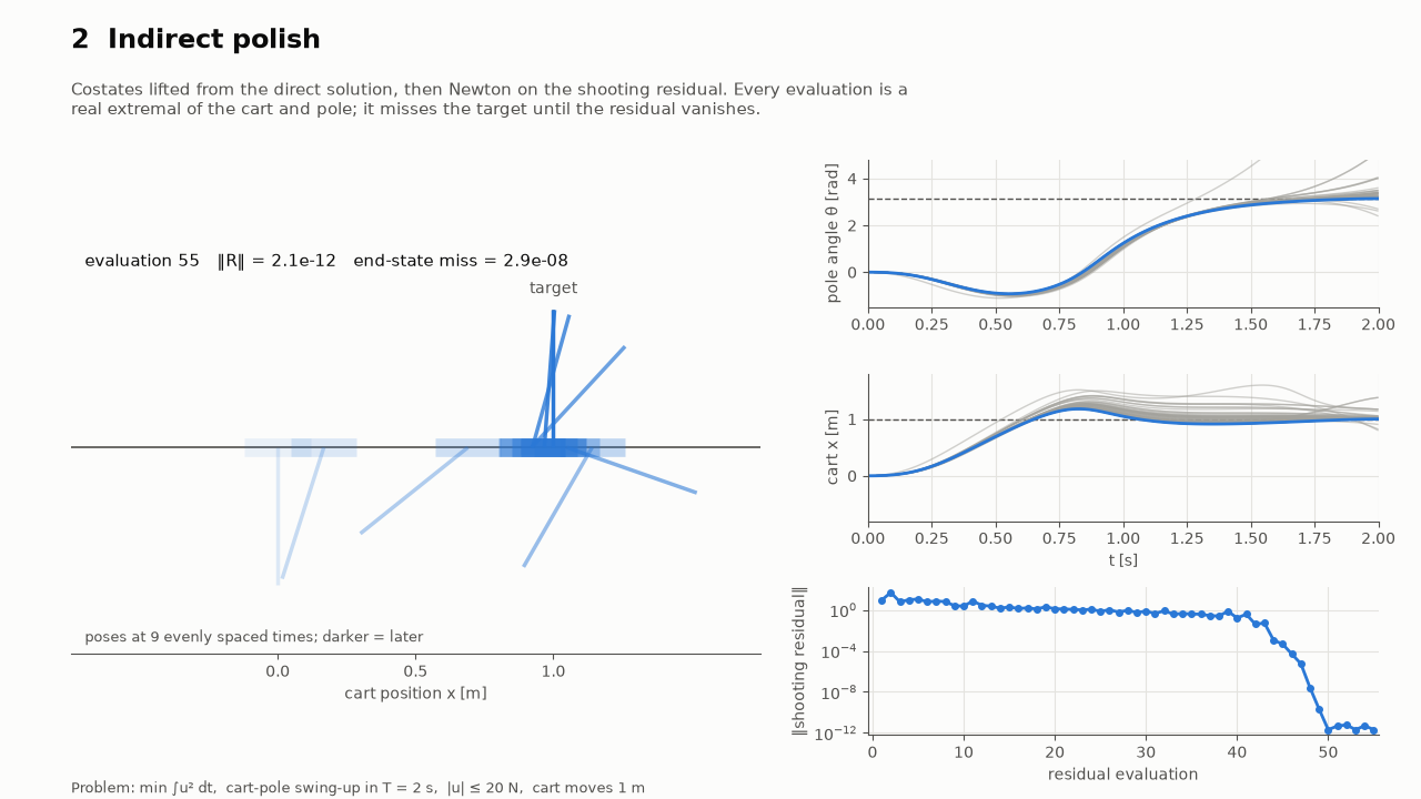
x = 1.18, withJ = 58.808. Polishing it indirectly reproduces the published value. Random costate search finds a different extremal that never passesx = 1, withJ = 57.945, 1.5% cheaper. Driving SciPy's integrator on Kelly's equations with that control history confirms it reaches the target with that cost. Indirect search over costate space found a better local optimum than the published one.
Watching the solves
benchmarks/animate.py records how a benchmark is solved and renders it as
an animation. Every frame is a recorded solver iterate. It needs the viz
dependency group, plus ffmpeg for MP4 or Pillow (included) for GIF:
uv run --group viz python benchmarks/animate.py cart_pole --stills   # outputs/cart_pole.mp4
uv run --group viz python benchmarks/animate.py earth_mars --stills
uv run --group viz python benchmarks/animate.py bryson_denham --stills
uv run --group viz python benchmarks/animate.py velocity_limit --stills
uv run --group viz python benchmarks/animate.py speed_limit --stills
uv run --group viz python benchmarks/animate.py cart_pole --reuse --out outputs/cart_pole.gif
Recording runs the solves (seconds to about a minute) and saves
<out>.npz, so --reuse re-renders without solving. Each animation opens
with a card stating the problem (story, formulation, how it is solved) and
keeps a one-line summary at the bottom. The rendered videos are in
docs/visuals/.
- Cart-pole (
cart_pole.mp4):- Kelly's direct-method iterates, from a dynamically infeasible straight-line guess.
- Every Newton evaluation of the indirect polish. Each is a real swing-up that misses the target until the residual vanishes.
- Random costate search, where every converged start finds the cheaper extremal.
- Both extremals swinging up side by side.
- Earth–Mars (
earth_mars.mp4):- Energy-optimal shooting from random costates, showing every Newton evaluation of the winning start as a real flight from Earth.
- The energy-to-fuel continuation, with the throttle sharpening into bang-bang and the arrival mass rising.
- The exact fuel-optimal flight: Earth, Mars and the spacecraft moving, with the switching function deciding thrust and coast.
- Bryson–Denham (
bryson_denham.mp4), for the touch regime and then the boundary-arc regime:- Penalty continuation in ρ pushing the mass back to the wall, with the cost climbing to the closed form from below.
- The exact multi-arc solve seeded from it, with the costate jump at the contact.
- Both solutions moving against their walls.
- Elevator: speed and force limits (
velocity_limit.mp4), exact arcs with a clipped control:- Penalty continuation on the speed limit, with the force clipped
exactly at
|u| ≤ 8throughout. - The exact multi-arc solve: full force, a ramp onto the limit, the limit, the mirror image.
- The move, beside the same move without the force limit.
- Penalty continuation on the speed limit, with the force clipped
exactly at
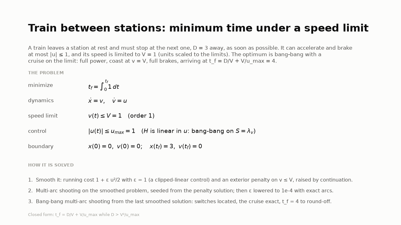
- Train between stations (
speed_limit.mp4), minimum time, exact arcs with a bang-bang control:- The smoothed problem (
1 + ε u²/2) under penalty continuation. - Smoothing continuation with exact arcs,
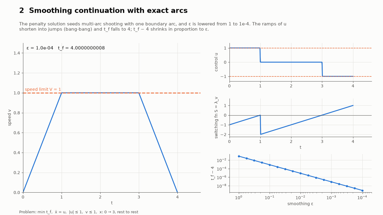
εfrom 1 to 1e-4: the ramps sharpen into jumps andt_f − 4shrinks withε. - The bang-bang exact solve: full power, cruise on the limit, brakes,
t_f = 4to round-off. - The run, beside the run without a speed limit.
- The smoothed problem (
 |
 |
 |
 |
 |
 |
Limitations
- Singular arcs are not handled: where a switching function stays at zero over an interval, the control takes its lower bound.
- Saturation corners and switches carry the tolerance. The corners of a clipped (quadratic, bounded) control are kinks in the dynamics. Like bang-bang switches, they are located and the integration restarts there. The state at a restart comes from the dense output of the step that found it, so it carries that step's error, at the integration tolerance.
- Tangential switches (
dS/dt = 0at the switch) have no jump and stop propagation with status-3. - Exact arcs need the structure.
MultiArcShootingsolves a given sequence of boundary arcs and touch points. Find it from a penalty solution, or for bang-bang controls from a smoothed problem. Not supported with exact arcs: unit-vector control sets, limits that depend explicitly on time (Hthen jumps at the entry), order 3 or more, singular arcs, and two constraints active at once. - Order-1 entries with a smooth control converge linearly. There
Hcontinuity has a double root (the control is continuous, soHdiffers only to second order), so Newton converges linearly and junction times come out to about 1e-8 while the cost is exact to 1e-12 or better. - Single shooting and large penalties. Penalty continuation gets
ill-conditioned as the weight grows (about
exp(sqrt(rho) T)): around ρ = 400 for the velocity limit, 3e7 for Bryson–Denham's boundary arc. Exact arcs do not need large weights, only a penalty solution good enough to read the structure from.
Developing against a local fast-numerical-integration
CI and normal installs use FNI from PyPI, pinned in uv.lock. To try changes
to a local FNI checkout (here a sibling directory):
-
One-off: run anything against the local checkout without touching the lockfile. uv builds the local copy in an overlay environment.
uv run --with-editable ../fast-numerical-integration pytest
-
Persistent: add this to
pyproject.toml, thenuv sync:[tool.uv.sources] fast-numerical-integration = { path = "../fast-numerical-integration", editable = true }
This rewrites
uv.lockto point at the path, so don't commit either change. Release the FNI change to PyPI, bump the requirement here and runuv lock --upgrade-package fast-numerical-integrationinstead.
Releasing
Releases are published from GitHub Actions (.github/workflows/release.yml)
with PyPI trusted publishing, so no tokens are stored.
- Bump
versioninpyproject.tomland merge the change tomain. - Optional rehearsal: run the Release workflow manually with
target: testpypi. - Tag and push:
git tag vX.Y.Z && git push origin vX.Y.Z. The workflow checks that the tag matches the version, builds the sdist and wheel, installs the wheel into a clean environment, runs the test suite against it, and uploads to PyPI.
Roadmap
Symbolic problem definition and Pontryagin derivationGenerated C kernels, compiled and wrapped for FNIState transition matrix, with jumps at switches; parameter sensitivitiesLiterature benchmarks: orbit raising, Earth–Mars, COPS robot arm, cart-pole, brachistochrone. Next: modified equinoctial elements and many-revolution transfers (Earth–Dionysus, GTO–GEO), and minimum-time attitude slews.Path constraints: order, exterior penalty with located crossings, termination; exact boundary arcs and touch points for order 1 and 2, with bounded and bang-bang controls. Next: singular arcs, and a control-continuity entry condition for order-1 limits.- Ways to choose initial costates, as separate optional layers on top of the
forward map:
single shooting and continuation; next, gradient-free search (PSO, differential evolution) and learned samplers of the costate space.
License
MIT; see LICENSE.
1 maintainer

Metadata
1 maintainer
Release files for auto-optimal-control 0.1.0
For a detailed explanation of source distributions (sdists) and built distributions (wheels), please see the package formats documentation.
Source distribution (sdist)
| File | Size | Uploaded | Provenance | Actions |
|---|---|---|---|---|
| auto_optimal_control-0.1.0.tar.gz | 106.7 kB | With provenance | Details for auto_optimal_control-0.1.0.tar.gz |
Built distribution (wheel)
| File | Interpreter | ABI | Platform | Actions Reset |
|---|---|---|---|---|
| auto_optimal_control-0.1.0-py3-none-any.whl | Python 3 | none | any | Details for auto_optimal_control-0.1.0-py3-none-any.whl |
Total release size: 173.1 kB
Release files / auto_optimal_control-0.1.0.tar.gz
| Download URL | auto_optimal_control-0.1.0.tar.gz |
|---|---|
| Size | 106.7 kB |
| Tags | Source |
|
SHA-256 checksum How to use checksums |
9ca109b788d8eb6faee08a47bc6ffc8f5126b8e5ffb0b6184bc0dcf9193225f7
|
|
BLAKE2b-256 checksum How to use checksums |
35db458a0510fe3fe04aa48f32e7ed450a3bd85ad207e1c508d44f92b2e887e6
|
| Upload date | |
|
Uploaded using Trusted Publishing? What is trusted publishing? |
Yes |
| Uploaded via |
twine/7.0.0 CPython/3.13.16
|
Provenance
Provenance describes where a file came from. On PyPI, provenance is shared via attestations, which provide a verifiable record of the build or publishing details. View details, limitations and caveats.


PyPI Publish Attestation
PyPI verified that this artifact, at this checksum, originated from the publisher listed below.
Signed by GitHub Actions, verified by PyPI on Nov 4, 2026.
Transparency logRelease files / auto_optimal_control-0.1.0-py3-none-any.whl
| Download URL | auto_optimal_control-0.1.0-py3-none-any.whl |
|---|---|
| Size | 66.4 kB |
| Tags | Python 3 |
|
SHA-256 checksum How to use checksums |
92688c44176098c358d55d81e9c5d8884718d756f6657562dcce70488a371e99
|
|
BLAKE2b-256 checksum How to use checksums |
cb094cf6c5440c72c80ead0c18b182c7d129c7c88fd57207e9efd91a6e9d2ecb
|
| Upload date | |
|
Uploaded using Trusted Publishing? What is trusted publishing? |
Yes |
| Uploaded via |
twine/7.0.0 CPython/3.13.16
|
Provenance
Provenance describes where a file came from. On PyPI, provenance is shared via attestations, which provide a verifiable record of the build or publishing details. View details, limitations and caveats.
PyPI Publish Attestation
PyPI verified that this artifact, at this checksum, originated from the publisher listed below.
Signed by GitHub Actions, verified by PyPI on Nov 4, 2026.
Transparency logSecurity for auto-optimal-control 0.1.0
Provenance
Provenance describes where a file came from. On PyPI, provenance is shared via attestations, which provide a verifiable record of the build or publishing details. View details, limitations and caveats.
Full provenance
All 2 files in this release have been uploaded with provenance metadata.
Attestation for auto_optimal_control-0.1.0.tar.gz
PyPI Publish Attestation
PyPI verified that this artifact, at this checksum, originated from the publisher listed below.
Signed by GitHub Actions, verified by PyPI on Nov 4, 2026.
Transparency logA note on package security
PyPI is a repository for distributing packages, not a service for auditing them. While third-party security researchers and our staff do their best to detect and remove malicious packages, PyPI cannot guarantee the quality, security or suitability of any given package.
To learn more about protecting yourself from malicious actors, visit our package security documentation.













