
BayesFilter
BayesFilter is a Python library for Bayesian filtering and smoothing. This library provides tools for implementing Bayesian filters, Rauch-Tung-Striebel smoothers, and other related methods. The only dependency is NumPy.
Installation
Install the released package from PyPI:
python -m pip install bayesfilter
For local development, install the package with its test dependencies:
python -m pip install -e '.[test]'
Constant-velocity example
The state below contains one-dimensional position and velocity. Observations measure position only.
import numpy as np

from bayesfilter.distributions import Gaussian
from bayesfilter.filtering import BayesianFilter
from bayesfilter.model import StateTransitionModel
from bayesfilter.observation import Observation
from bayesfilter.smoothing import RTS


def transition(state, delta_t_s):
    position, velocity = state
    return np.array([position + delta_t_s * velocity, velocity])


def transition_jacobian(_state, delta_t_s):
    return np.array([
        [1.0, delta_t_s],
        [0.0, 1.0],
    ])


def observe_position(state):
    return np.array([state[0]])


def observation_jacobian(_state):
    return np.array([[1.0, 0.0]])


transition_model = StateTransitionModel(
    transition_func=transition,
    transition_noise_covariance=np.diag([0.01, 0.001]),
    transition_jacobian_func=transition_jacobian,
)
initial_state = Gaussian(
    mean=np.array([0.0, 1.0]),
    covariance=np.diag([1.0, 0.25]),
)
bayes_filter = BayesianFilter(transition_model, initial_state)

rng = np.random.default_rng(0)
observation_times = np.arange(0.0, 10.5, 0.5)
position_measurements = observation_times + rng.normal(
    loc=0.0,
    scale=0.5,
    size=len(observation_times),
)
observations = [
    Observation(
        observation=np.array([position]),
        noise_covariance=np.array([[0.5**2]]),
        observation_func=observe_position,
        jacobian_func=observation_jacobian,
    )
    for position in position_measurements
]

filter_states, filter_times = bayes_filter.run(
    observations,
    observation_times,
    rate_hz=20.0,
    use_jacobian=True,
)

smoother_states = RTS(bayes_filter).apply(
    filter_states,
    filter_times,
    use_jacobian=True,
)
BayesianFilter.run() evaluates the model on its own fixed-rate time grid and
returns that grid as filter_times. Always pass filter_times, rather than the
original observation timestamps, to RTS.apply(). This matters whenever the
transition depends on delta_t_s.
As a convenience, filtering and smoothing can be run together:
bayes_filter = BayesianFilter(transition_model, initial_state)
smoother_states = RTS(bayes_filter).smooth(
    observations,
    observation_times,
    rate_hz=20.0,
    use_jacobian=True,
)
Use the explicit run() followed by apply() form when the corresponding
filter timestamps are also needed.
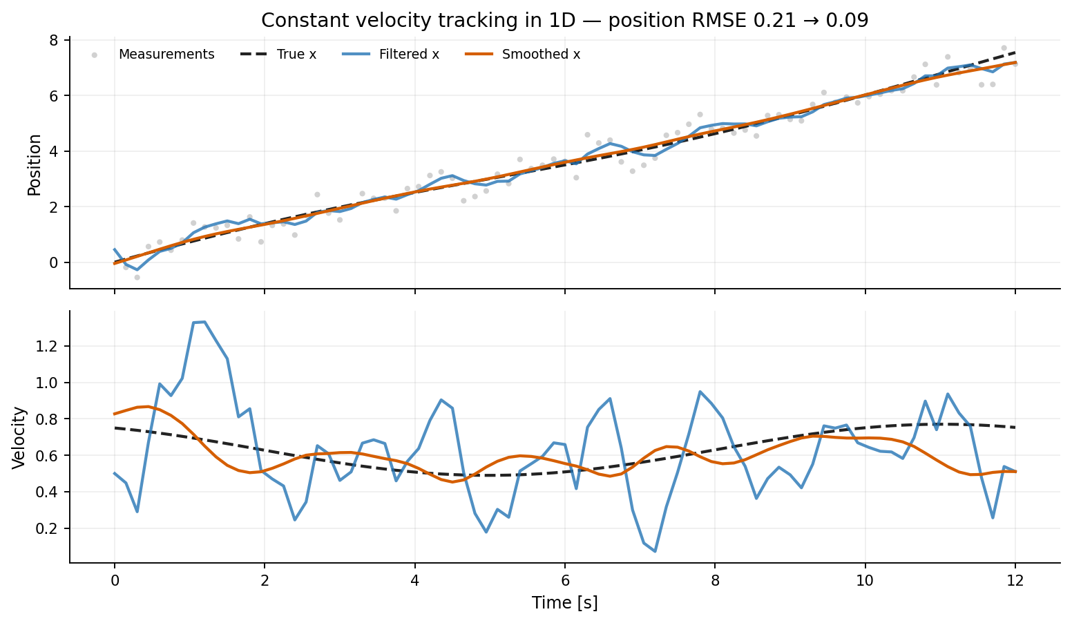
Noisy position measurements are filtered forward and then refined by the RTS smoother; velocity is inferred without being observed directly.
Jacobian and unscented modes
Set use_jacobian=True on filtering and smoothing calls to use the supplied
transition and observation Jacobians. Both Jacobian functions are required in
this mode.
Set use_jacobian=False to use unscented propagation. Jacobian functions may
then be omitted:
filter_states, filter_times = bayes_filter.run(
    observations,
    observation_times,
    rate_hz=20.0,
    use_jacobian=False,
)
For a Jacobian transition with covariance P and transition matrix F, the
predicted covariance and state-to-prediction cross-covariance are
P_pred = F @ P @ F.T + Q
cross_cov = P @ F.T
The RTS smoother gain is therefore
G = cross_cov @ inv(P_pred)
The unscented path obtains the corresponding cross-covariance directly from the propagated sigma points.
Synchronous observations
When there is exactly one observation per transition interval, use
run_synchronous():
states = bayes_filter.run_synchronous(
    observations,
    times_s,
    use_jacobian=True,
)
For N timestamps this method consumes at most N - 1 observations and
returns the initial state followed by each updated state. Use run() for
irregularly timed observations or when several observations may fall within a
single filter interval.
Covariance conventions
All noise arguments are covariance matrices, not standard deviations. For a
scalar measurement with standard deviation sigma, use
np.array([[sigma**2]]).
The transition noise covariance is added once per prediction performed by the filter. Observation covariances are added during their corresponding updates.
Examples
The examples generate deterministic synthetic observations, run a Bayesian
filter and RTS smoother, print quantitative errors, and save Matplotlib figures
under examples/figures/.
Install Matplotlib separately when running the examples:
python -m pip install -e .
python -m pip install -r examples/requirements.txt
Matplotlib is not a BayesFilter runtime dependency.
Running the examples
| Model | State | Command |
|---|---|---|
| Constant velocity, 1D | [p, v] |
python -m examples.constant_velocity_1d |
| Constant velocity, 2D | [pₓ, pᵧ, vₓ, vᵧ] |
python -m examples.constant_velocity_2d |
| Constant velocity, 3D | [p, v], with three-vectors |
python -m examples.constant_velocity_3d |
| Planar trajectory tracking | [pₓ, pᵧ, vₓ, vᵧ] |
python -m examples.planar_trajectory_tracking |
| Bearings-only target tracking | [pₓ, pᵧ, vₓ, vᵧ] |
python -m examples.bearings_only_tracking |
| Heading-coupled tracking | [pₓ, pᵧ, ψ, v, κ] |
python -m examples.heading_coupled_tracking |
| Constant acceleration, 1D | [p, v, a] |
python -m examples.constant_acceleration_1d |
| Constant acceleration, 2D | [p, v, a], with two-vectors |
python -m examples.constant_acceleration_2d |
| Constant acceleration, 3D | [p, v, a], with three-vectors |
python -m examples.constant_acceleration_3d |
| Rigid body, known inertia | [p, v, ϕ, ω] |
python -m examples.rigid_body_known_inertia |
| Rigid body, inferred inertia | [p, v, ϕ, ω, η₂, η₃] |
python -m examples.rigid_body_inertia_estimation |
Regenerate every figure, including the figure at the top of this README, with:
python -m examples.generate_figures
All examples use fixed random seeds. Their simulation functions can be imported without importing Matplotlib.
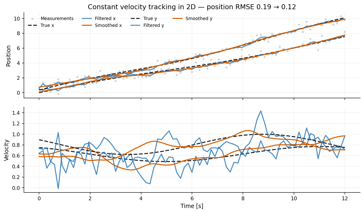
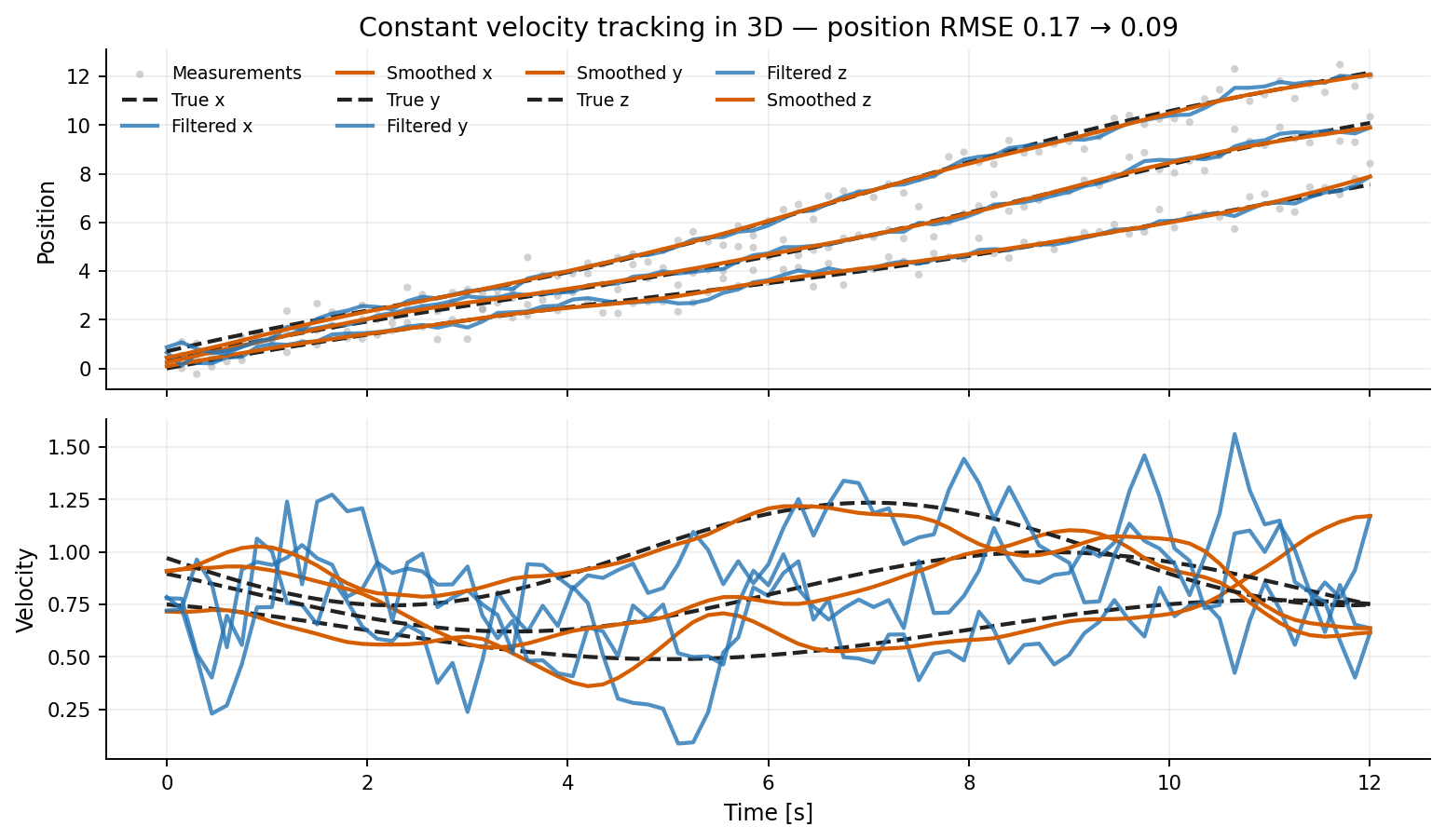
Constant-velocity tracking
For spatial dimension d, the state contains position and velocity:
x = [p, v]
The transition and position observation matrices are
F = [[I, dt I],
     [0,    I]]

H = [I, 0]
Process noise uses the discrete white-acceleration covariance
Q = q [[dt³/3, dt²/2],
       [dt²/2,    dt]] ⊗ I.
| 1D | 2D | 3D |
|---|---|---|
 |
 |
 |
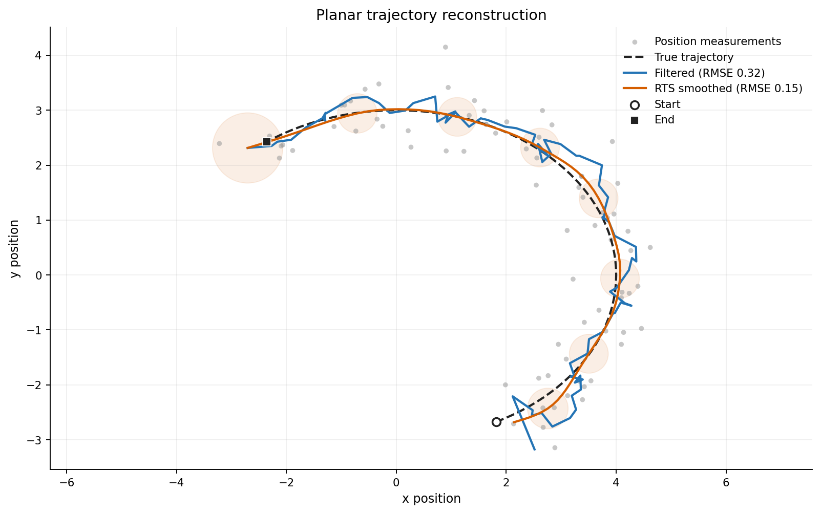
The same position-and-velocity state can reconstruct a curved planar trajectory. The ellipses below show selected 95% smoothed position-confidence regions.
Bearings-only target tracking
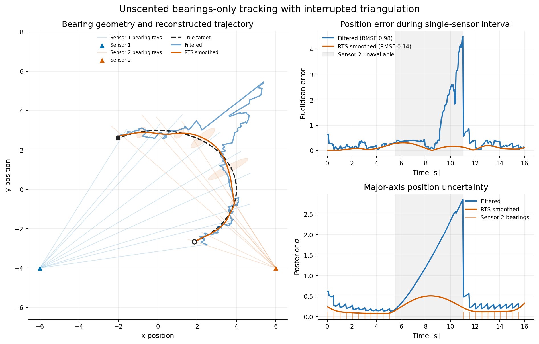
This example tracks a curved target without observing range or position directly. Two fixed sensors report noisy world-frame bearing unit vectors:
x = [pₓ, pᵧ, vₓ, vᵧ]

hᵢ(x) = (p - sᵢ) / ‖p - sᵢ‖,
where sᵢ is the position of sensor i. Encoding bearing as
[cos(bearing), sin(bearing)] avoids a discontinuous scalar residual at
±π. The observation remains strongly nonlinear and supplies no information
in the instantaneous line-of-sight direction.
Sensor 1 reports at 10 Hz. Sensor 2 reports at 2 Hz but is unavailable from 5.5–11 seconds. During that interval, range is only weakly observable from target motion, so the filtered uncertainty grows along the remaining bearing geometry. When sensor 2 returns, triangulation rapidly reduces it. The RTS smoother also uses those later measurements to reconstruct the dropout.
Heading-coupled planar tracking
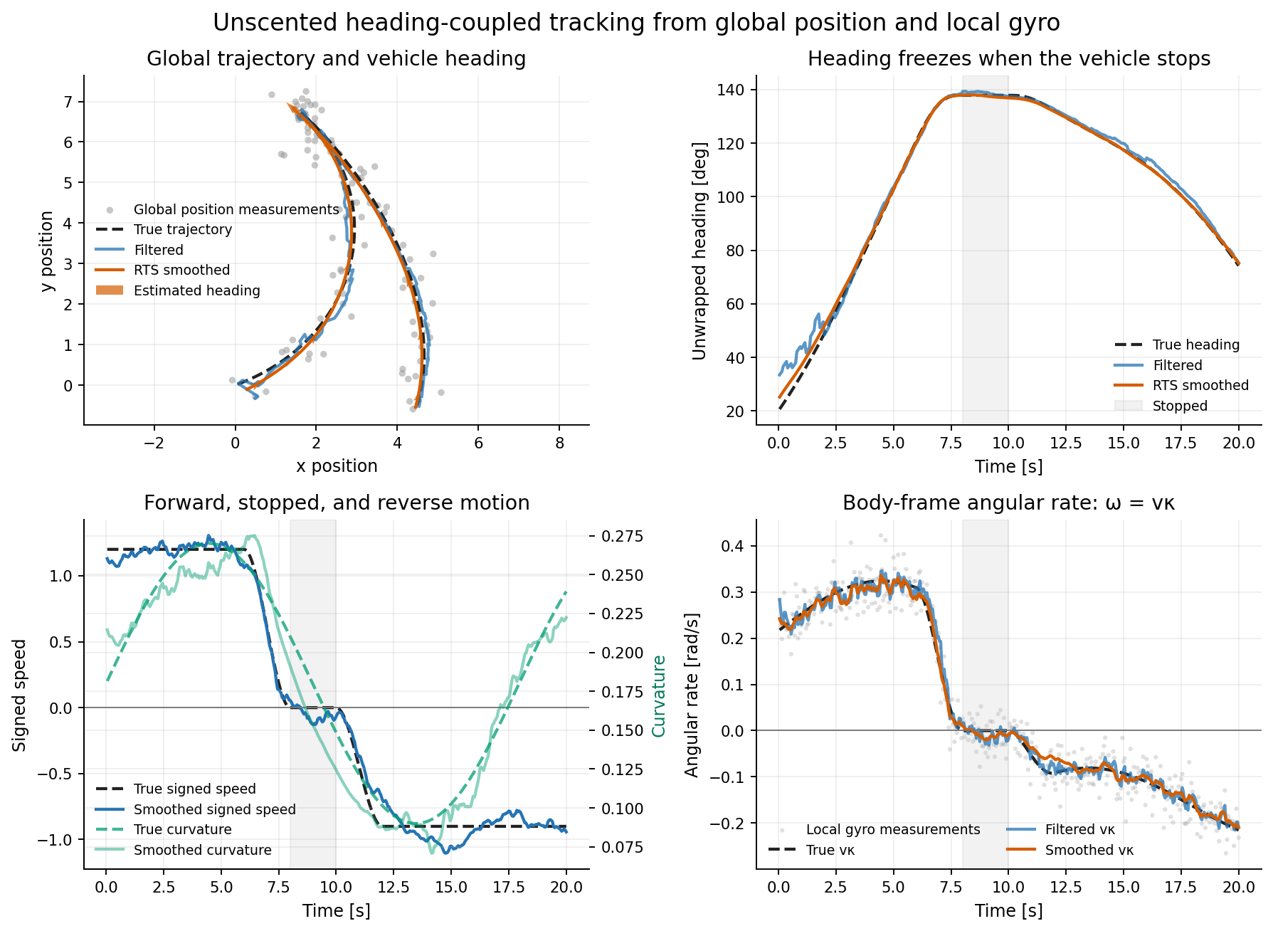
This example models a nonholonomic vehicle with state
x = [pₓ, pᵧ, ψ, v, κ],
where ψ is its unwrapped world heading, v is signed longitudinal speed,
and κ is signed curvature. Heading rate is coupled to motion:
ψ̇ = v κ.
The vehicle therefore cannot turn in place: both translation and heading rate
vanish when v = 0. Negative speed represents reversing and changes the sign
of the heading rate for fixed curvature. The discrete midpoint transition is
α = ψ + ½ dt v κ

pₓ' = pₓ + dt v cos(α)
pᵧ' = pᵧ + dt v sin(α)
ψ'  = ψ + dt v κ.
The filter asynchronously fuses noisy 5 Hz global position fixes with noisy 20 Hz body-frame angular-rate measurements:
z_position = [pₓ, pᵧ] + noise
z_gyro     = v κ + noise.
The deterministic trajectory drives forward, stops from 8–10 seconds, and then reverses. The default example uses unscented propagation; analytic Jacobians are also supplied and tested.
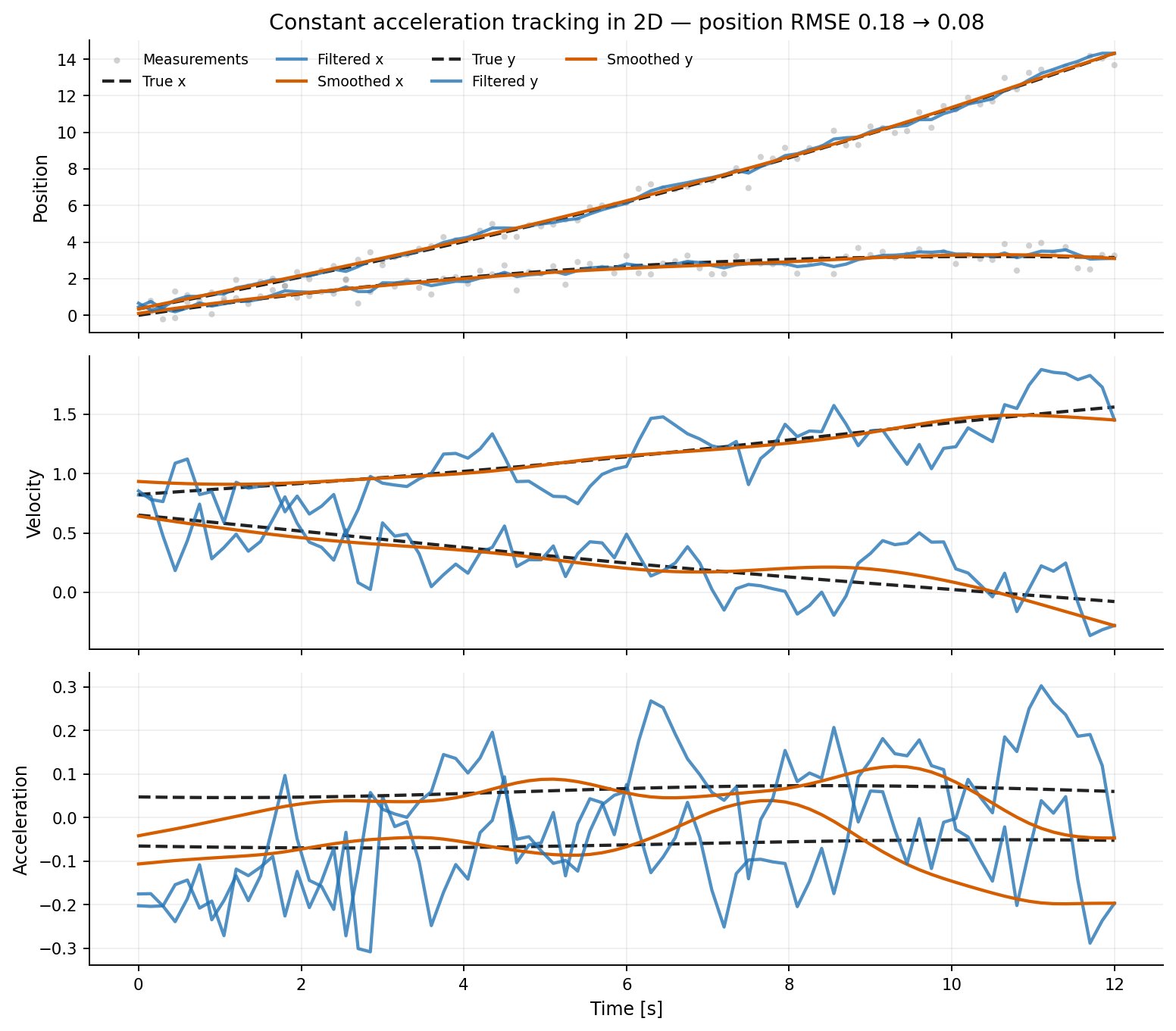
Constant-acceleration tracking
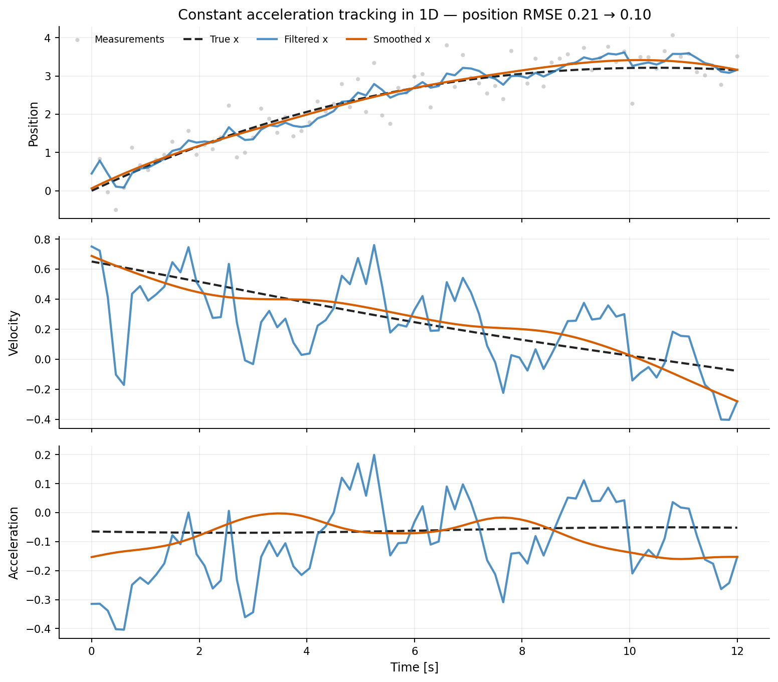
The state contains position, velocity, and acceleration:
x = [p, v, a]
Its transition is
F = [[I, dt I, ½ dt² I],
     [0,    I,     dt I],
     [0,    0,        I]].
Process noise uses the corresponding discrete white-jerk covariance. As in the velocity examples, noisy position is the only observed state component.
| 1D | 2D | 3D |
|---|---|---|
 |
 |
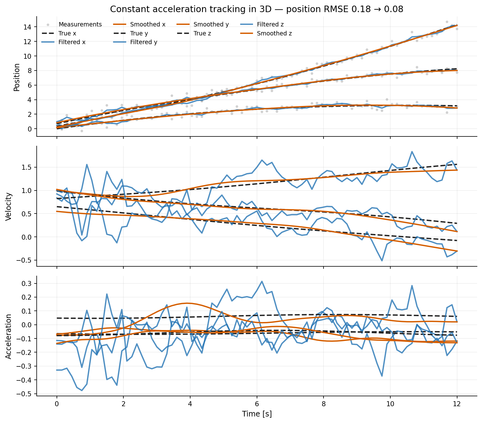 |
The current transition-model API stores one fixed process covariance. These
examples therefore use fixed-cadence synchronous observations and construct
Q for that cadence.
Rigid-body state and dynamics
The rigid-body state is
x = [p, v, ϕ, ω],
where p and v are world-frame center position and velocity, ω is
body-frame angular velocity, and ϕ ∈ R³ is a rotation bivector/vector. Its
equivalent representations are
R = Exp([ϕ]×)
q = Exp(½ [0, ϕ])
ϕ = 2 vec(Log(q)).
Translation follows constant velocity. Rotation follows the torque-free Euler
equation for a body with inertia matrix I:
I ω̇ + ω × (I ω) = 0.
Angular velocity is integrated with RK4. Attitude is advanced by composition on SO(3):
R_next = R Exp([dt ω_mid]×).
The state is then returned to bivector coordinates with Log(R_next). The
examples remain inside one principal-log chart and do not cross the π branch
boundary. BayesFilter does not yet provide manifold-aware Gaussian means or
retractions, so this chart restriction is intentional.
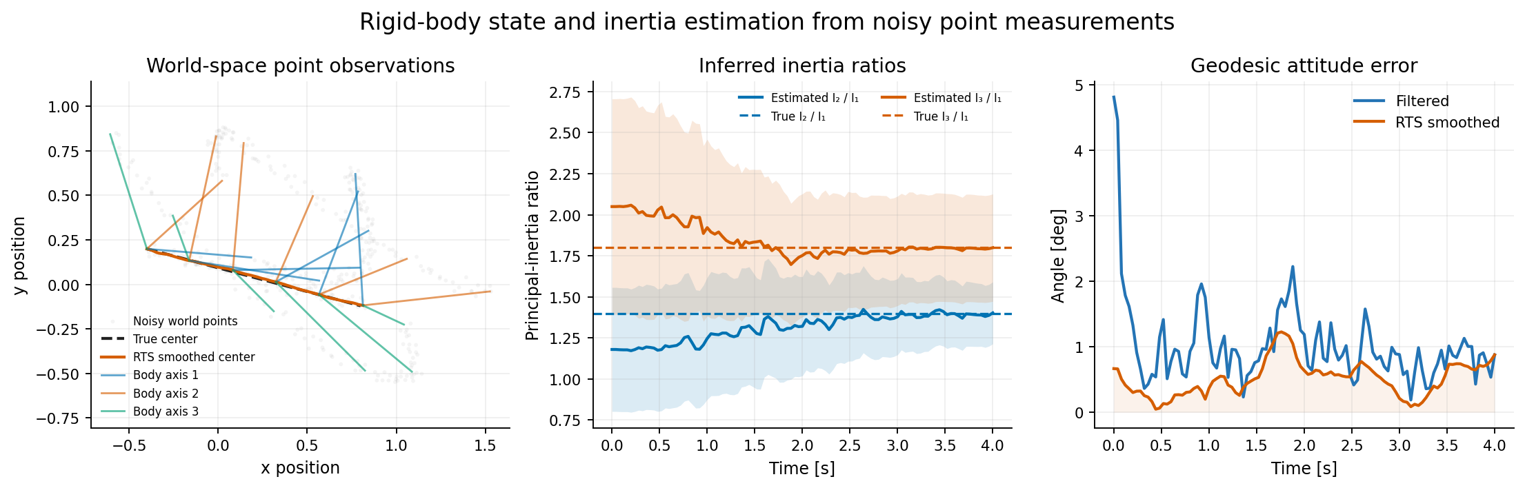
World-space point observations
The body carries four labeled canonical points:
c₀ = 0, c₁ = 0.75 e₁, c₂ = 0.75 e₂, c₃ = 0.75 e₃.
Their predicted world locations are
hᵢ(x) = p + R(ϕ)cᵢ.
The origin marker observes translation directly. Subtracting it from the other marker positions recovers scaled columns of the rotation matrix. The filter residual therefore lives in ordinary Cartesian point space; it never subtracts quaternions or rotation vectors directly.
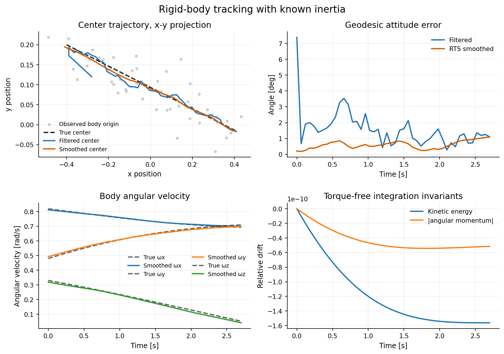
Known fixed inertia
The known-inertia example uses diag(1.0, 1.4, 1.8) and the unscented filter
and smoother. Its figure shows position tracking, geodesic attitude error,
body angular velocity, and numerical conservation of torque-free invariants.
Inferring inertia ratios in the state
Torque-free angular motion is unchanged if every principal moment is scaled
by the same constant. Absolute inertia scale is therefore unobservable from
these measurements. The augmented example fixes I₁ = 1 and estimates the
two identifiable log ratios
η₂ = log(I₂ / I₁), η₃ = log(I₃ / I₁).
Exponentiation keeps the inferred ratios positive. The parameters have tiny process noise and are inferred indirectly from the observed world-space point trajectories—there are no direct angular-velocity or inertia measurements. The default run uses 100 point-observation sets over four seconds, making both the ratio convergence and posterior-uncertainty contraction visible.
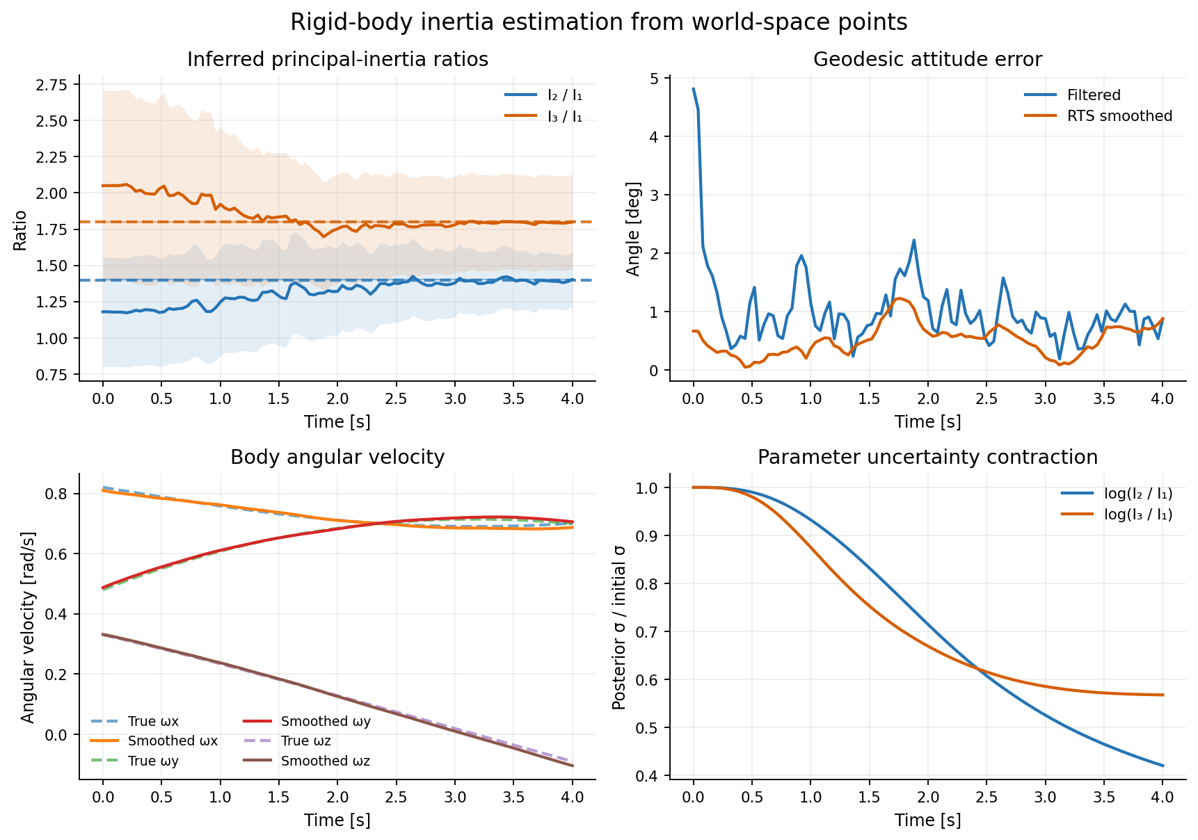
To identify absolute inertia scale, an example would need a known applied torque or another measurement that supplies scale information.
Tests
The suite contains analytic linear-Gaussian regression tests and integration tests covering filtering, smoothing, irregular observation timing, batched observations, and both propagation modes.
python -m pip install -e '.[test]'
python -m pytest
Pytest measures branch coverage for the bayesfilter package and enforces the
minimum configured in pytest.ini.
Package layout
bayesfilter/distributions.py: Gaussian distributions and sigma points.bayesfilter/model.py: State transition models.bayesfilter/observation.py: Observation models.bayesfilter/filtering.py: Bayesian prediction and update loops.bayesfilter/smoothing.py: RTS smoothing.bayesfilter/unscented.py: Unscented-transform utilities.examples/: Runnable tracking and rigid-body examples and their figures.tests/: Unit and integration tests.
License
BayesFilter is distributed under the MIT License. See LICENSE.
1 maintainer

Metadata
1 maintainer
Release files for bayesfilter 0.1.0
For a detailed explanation of source distributions (sdists) and built distributions (wheels), please see the package formats documentation.
Source distribution (sdist)
| File | Size | Uploaded | |
|---|---|---|---|
| bayesfilter-0.1.0.tar.gz | 3.2 MB | Details |
Built distribution (wheel)
| File | Interpreter | ABI | Platform | Reset |
|---|---|---|---|---|
| bayesfilter-0.1.0-py3-none-any.whl | Python 3 | none | any | Details |
Total release size: 3.2 MB
Release files / bayesfilter-0.1.0.tar.gz
| Download URL | bayesfilter-0.1.0.tar.gz |
|---|---|
| Size | 3.2 MB |
| Tags | Source |
|
SHA-256 checksum How to use checksums |
2fcad9220aaea883879331b3df48ae30aad6f0a825e468aecca3c99bd8e54686
|
|
BLAKE2b-256 checksum How to use checksums |
805bc1923f417c75d929deb253878ccf3ca45fd079d2736b002dee5eb7eb43a9
|
| Upload date | |
|
Uploaded using Trusted Publishing? What is trusted publishing? |
Yes |
| Uploaded via |
twine/7.0.0 CPython/3.13.14
|
Provenance
Provenance describes where a file came from. On PyPI, provenance is shared via attestations, which provide a verifiable record of the build or publishing details. View details, limitations and caveats.


PyPI Publish Attestation
PyPI verified that this artifact, at this checksum, originated from the publisher listed below.
Signed by GitHub Actions, verified by PyPI on Sep 11, 2026.
Transparency logRelease files / bayesfilter-0.1.0-py3-none-any.whl
| Download URL | bayesfilter-0.1.0-py3-none-any.whl |
|---|---|
| Size | 15.0 kB |
| Tags | Python 3 |
|
SHA-256 checksum How to use checksums |
76ca6c5834d3130d4dbe89019a6ca31ca0b3d1ec95729b65885f64e0b73ec61f
|
|
BLAKE2b-256 checksum How to use checksums |
e1a4953cafdd1316db81a20551884a9d00cf94bf54afe4993562dc349b09f48e
|
| Upload date | |
|
Uploaded using Trusted Publishing? What is trusted publishing? |
Yes |
| Uploaded via |
twine/7.0.0 CPython/3.13.14
|
Provenance
Provenance describes where a file came from. On PyPI, provenance is shared via attestations, which provide a verifiable record of the build or publishing details. View details, limitations and caveats.
PyPI Publish Attestation
PyPI verified that this artifact, at this checksum, originated from the publisher listed below.
Signed by GitHub Actions, verified by PyPI on Sep 11, 2026.
Transparency log













