
BayesFilter
BayesFilter is a Python library for Bayesian filtering and smoothing. This library provides tools for implementing Bayesian filters, Rauch-Tung-Striebel smoothers, and other related methods. The only dependency is NumPy.
Installation
Install the released package from PyPI:
python -m pip install bayesfilter
For local development, install the package with its test dependencies:
python -m pip install -e '.[test]'
Constant-velocity example
The state below contains one-dimensional position and velocity. Observations measure position only.
import numpy as np

from bayesfilter.distributions import Gaussian
from bayesfilter.filtering import BayesianFilter
from bayesfilter.model import StateTransitionModel
from bayesfilter.observation import Observation
from bayesfilter.smoothing import RTS


def transition(state, delta_t_s):
    position, velocity = state
    return np.array([position + delta_t_s * velocity, velocity])


def transition_jacobian(_state, delta_t_s):
    return np.array([
        [1.0, delta_t_s],
        [0.0, 1.0],
    ])


def observe_position(state):
    return np.array([state[0]])


def observation_jacobian(_state):
    return np.array([[1.0, 0.0]])


transition_model = StateTransitionModel(
    transition_func=transition,
    transition_noise_covariance=np.diag([0.01, 0.001]),
    transition_jacobian_func=transition_jacobian,
)
initial_state = Gaussian(
    mean=np.array([0.0, 1.0]),
    covariance=np.diag([1.0, 0.25]),
)
bayes_filter = BayesianFilter(transition_model, initial_state)

rng = np.random.default_rng(0)
observation_times = np.arange(0.0, 10.5, 0.5)
position_measurements = observation_times + rng.normal(
    loc=0.0,
    scale=0.5,
    size=len(observation_times),
)
observations = [
    Observation(
        observation=np.array([position]),
        noise_covariance=np.array([[0.5**2]]),
        observation_func=observe_position,
        jacobian_func=observation_jacobian,
    )
    for position in position_measurements
]

filter_states, filter_times = bayes_filter.run(
    observations,
    observation_times,
    rate_hz=20.0,
    use_jacobian=True,
)

smoother_states = RTS(bayes_filter).apply(
    filter_states,
    filter_times,
    use_jacobian=True,
)
BayesianFilter.run() evaluates the model on its own fixed-rate time grid and
returns that grid as filter_times. Always pass filter_times, rather than the
original observation timestamps, to RTS.apply(). This matters whenever the
transition depends on delta_t_s.
As a convenience, filtering and smoothing can be run together:
bayes_filter = BayesianFilter(transition_model, initial_state)
smoother_states = RTS(bayes_filter).smooth(
    observations,
    observation_times,
    rate_hz=20.0,
    use_jacobian=True,
)
Use the explicit run() followed by apply() form when the corresponding
filter timestamps are also needed.
Noisy position measurements are filtered forward and then refined by the RTS smoother; velocity is inferred without being observed directly.
Jacobian and unscented modes
Set use_jacobian=True on filtering and smoothing calls to use the supplied
transition and observation Jacobians. Both Jacobian functions are required in
this mode.
Set use_jacobian=False to use unscented propagation. Jacobian functions may
then be omitted:
filter_states, filter_times = bayes_filter.run(
    observations,
    observation_times,
    rate_hz=20.0,
    use_jacobian=False,
)
For a Jacobian transition with covariance P and transition matrix F, the
predicted covariance and state-to-prediction cross-covariance are
P_pred = F @ P @ F.T + Q
cross_cov = P @ F.T
The RTS smoother gain is therefore
G = cross_cov @ inv(P_pred)
The unscented path obtains the corresponding cross-covariance directly from the propagated sigma points.
Synchronous observations
When there is exactly one observation per transition interval, use
run_synchronous():
states = bayes_filter.run_synchronous(
    observations,
    times_s,
    use_jacobian=True,
)
For N timestamps this method consumes at most N - 1 observations and
returns the initial state followed by each updated state. Use run() for
irregularly timed observations or when several observations may fall within a
single filter interval.
Covariance conventions
All noise arguments are covariance matrices, not standard deviations. For a
scalar measurement with standard deviation sigma, use
np.array([[sigma**2]]).
The transition noise covariance is added once per prediction performed by the filter. Observation covariances are added during their corresponding updates.
Examples
The examples generate deterministic synthetic observations, run a Bayesian
filter and RTS smoother, print quantitative errors, and save Matplotlib figures
under examples/figures/.
Install Matplotlib separately when running the examples:
python -m pip install -e .
python -m pip install -r examples/requirements.txt
Matplotlib is not a BayesFilter runtime dependency.
Choose an example
Start with the foundations, then choose a category according to the kind of model, sensor geometry, or unknown parameter you want to explore. Every row links to a detailed walkthrough below.
Foundations
| Model | State | Command |
|---|---|---|
| Constant velocity, 1D | [p, v] |
python -m examples.constant_velocity_1d |
| Constant velocity, 2D | [pₓ, pᵧ, vₓ, vᵧ] |
python -m examples.constant_velocity_2d |
| Constant velocity, 3D | [p, v], with three-vectors |
python -m examples.constant_velocity_3d |
| Constant acceleration, 1D | [p, v, a] |
python -m examples.constant_acceleration_1d |
| Constant acceleration, 2D | [p, v, a], with two-vectors |
python -m examples.constant_acceleration_2d |
| Constant acceleration, 3D | [p, v, a], with three-vectors |
python -m examples.constant_acceleration_3d |
| Planar trajectory tracking | [pₓ, pᵧ, vₓ, vᵧ] |
python -m examples.planar_trajectory_tracking |
| Heading-coupled planar motion | [pₓ, pᵧ, ψ, v, κ] |
python -m examples.heading_coupled_tracking |
Nonlinear tracking and localization
| Model | State | Command |
|---|---|---|
| Bearings-only target tracking | [pₓ, pᵧ, vₓ, vᵧ] |
python -m examples.bearings_only_tracking |
| Radar + camera target fusion | [pₓ, pᵧ, vₓ, vᵧ] |
python -m examples.radar_camera_fusion |
| TDOA emitter localization | [pₓ, pᵧ, vₓ, vᵧ, b₂, …, b₅] |
python -m examples.tdoa_emitter_localization |
| Doppler-only source localization | [sₓ, sᵧ, f₀] |
python -m examples.doppler_source_localization |
| Ballistic radar tracking and drag inference | [x, h, vₓ, vₕ, log(c_d)] |
python -m examples.ballistic_tracking |
Navigation and mapping
| Model | State | Command |
|---|---|---|
| Local/global vehicle fusion | [x, y, ψ, v, ω, b_g] |
python -m examples.local_global_fusion |
| Black-box INS and GPS fusion | [t_GL, ψ_GL, v_drift, ω_drift] |
python -m examples.ins_gps_fusion |
| Sun-aided island navigation | [p, ψ, v, ω, c] |
python -m examples.boat_navigation |
| Boat current and compass-bias inference | [x, y, ψ, v, ω, cₓ, cᵧ, b] |
python -m examples.boat_current_compass_bias |
| Known-correspondence landmark SLAM | [pₓ, pᵧ, ψ, v, ω, ℓ₁, …, ℓ₈] |
python -m examples.known_correspondence_slam |
| Aircraft bank from position tracks | [x, y, z, v, χ, γ, ϕ] |
python -m examples.aircraft_bank_inference |
Space and orbital estimation
| Model | State | Command |
|---|---|---|
| Orbit determination from ground stations | [rₓ, rᵧ, vₓ, vᵧ] |
python -m examples.orbit_determination |
| Angles-only asteroid orbit determination | [x, y, vₓ, vᵧ] |
python -m examples.asteroid_orbit |
| Planet mass from a spacecraft flyby | [x, y, vₓ, vᵧ, log(μ)] |
python -m examples.planet_flyby_mass |
Rigid-body and inertial estimation
| Model | State | Command |
|---|---|---|
| Rigid body, known inertia | [p, v, ϕ, ω] |
python -m examples.rigid_body_known_inertia |
| Rigid body, inferred inertia | [p, v, ϕ, ω, η₂, η₃] |
python -m examples.rigid_body_inertia_estimation |
| Gravity vector from raw IMU | [g_b, ω] |
python -m examples.gravity_vector_from_imu |
| Phone gyrocompassing | [Ωₘ, b_g] |
python -m examples.phone_gyrocompass |
Sensor and geometric calibration
| Model | State | Command |
|---|---|---|
| Camera/gyro spatiotemporal calibration | [ϕ_CG, Δt, b_g] |
python -m examples.camera_gyro_calibration |
| Wrist-camera hand-eye calibration | [t_WC, ϕ_WC, t_BO, ϕ_BO] |
python -m examples.wrist_camera_hand_eye_calibration |
| GNSS lever-arm calibration | [x, y, ψ, v, ω, ℓₓ, ℓᵧ] |
python -m examples.gnss_lever_arm_calibration |
| IMU lever-arm calibration | [r, b_a] |
python -m examples.imu_lever_arm_calibration |
| Wheel-radius and speedometer calibration | [p, v, a, log(r), b] |
python -m examples.vehicle_wheel_calibration |
Physical parameter inference
| Model | State | Command |
|---|---|---|
| Battery charge and resistance | [q, vₚ, log(R₀), I] |
python -m examples.battery_state_of_charge |
| House thermal parameters | [T, log(R), log(C)] |
python -m examples.thermal_house |
| Pendulum parameters | [θ, θ̇, log(L), log(c)] |
python -m examples.pendulum_parameter_inference |
| Bouncing-ball parameters | [z, v, log(c_d), logit(e)] |
python -m examples.bouncing_ball_parameter_inference |
| Sloshing fill level | [q, q̇, h, ḣ, a_tank] |
python -m examples.sloshing_fill_level |
| Active-suspension road profile | [z_s, v_s, z_u, v_u, r, ṙ, log(k), log(c), F] |
python -m examples.active_suspension_road_profile |
| Vehicle coast-down parameters | [v, Cᵣᵣ, C_d A] |
python -m examples.vehicle_coastdown |
| Wheel-slip estimation | [p, v, a, logit(s)] |
python -m examples.wheel_slip_estimation |
Measurement-model lessons
| Model | State | Command |
|---|---|---|
| Quantization-noise covariance | [θ, θ̇] |
python -m examples.quantization_noise |
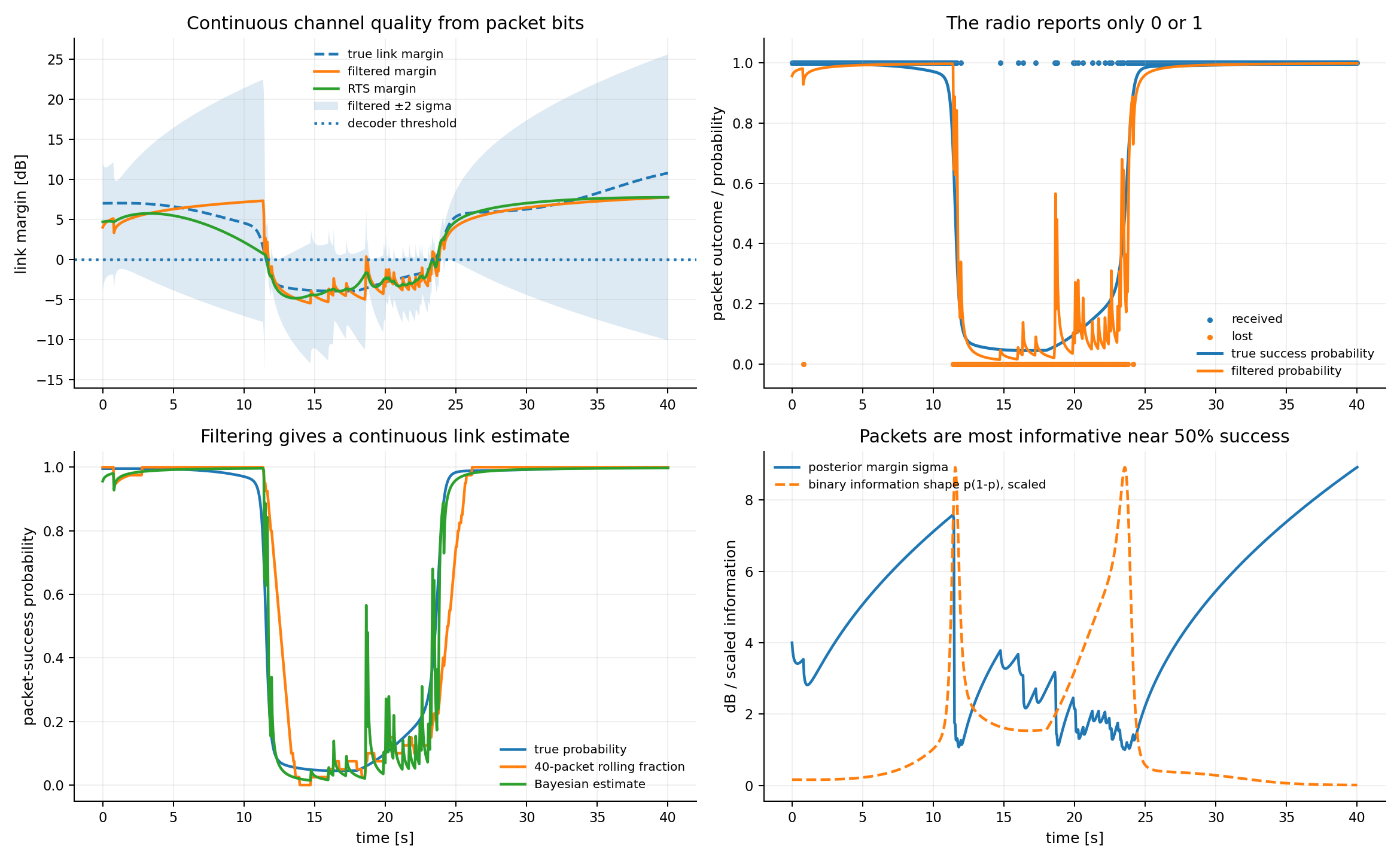
| Binary-packet channel tracking | [link margin] |
python -m examples.binary_packet_channel |
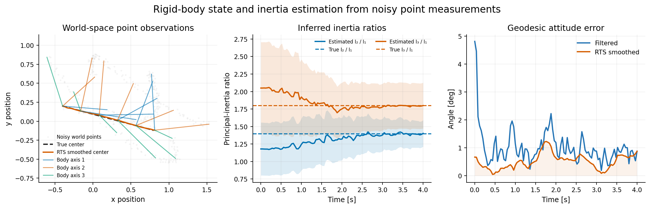
Regenerate every figure, including the figure at the top of this README, with:
python -m examples.generate_figures
All examples use fixed random seeds. Their simulation functions can be imported without importing Matplotlib.
Example walkthroughs
The walkthroughs follow the same progression as the directory above: from linear motion models to nonlinear sensing, navigation, calibration, physical parameter inference, and focused measurement-model lessons.
Foundations
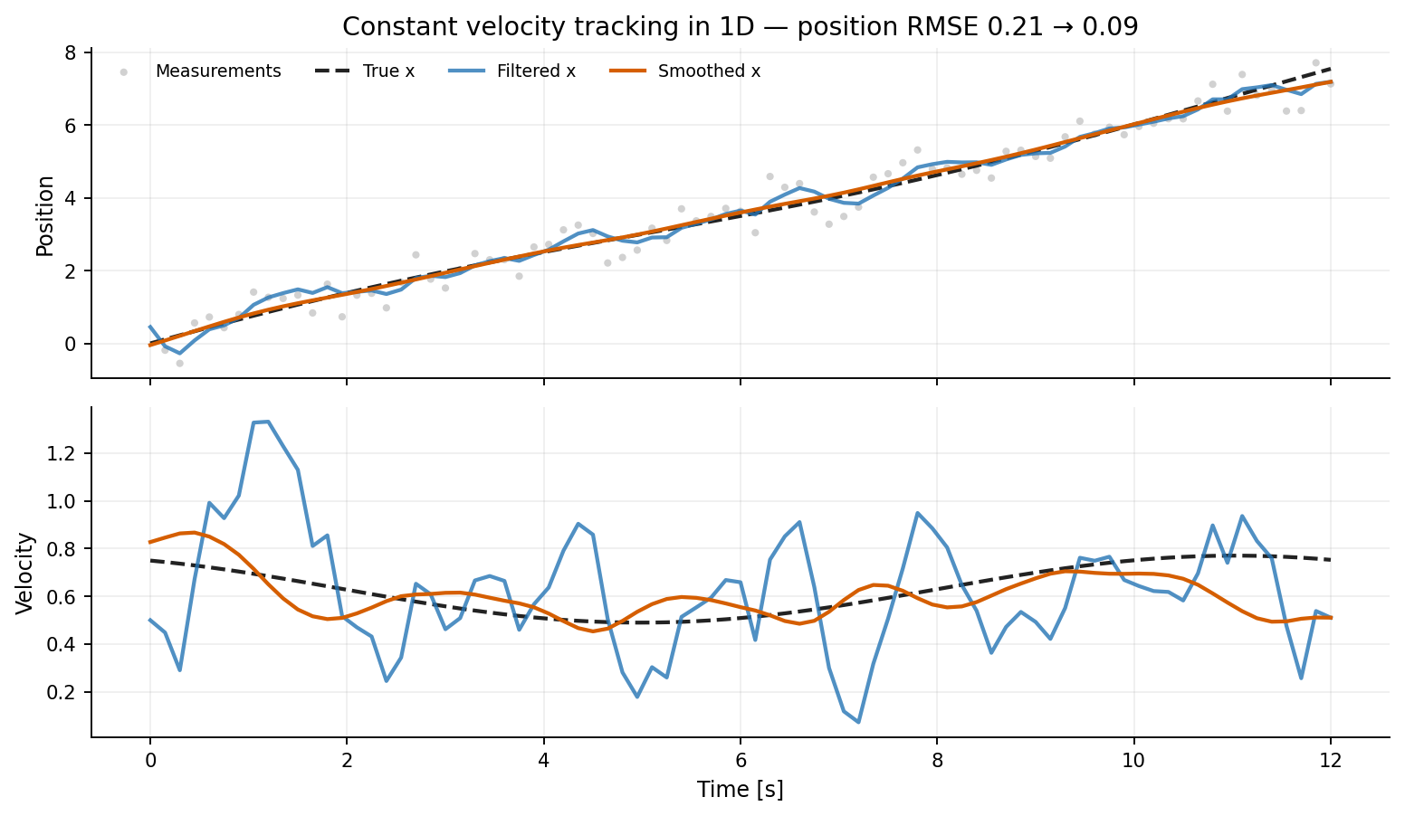
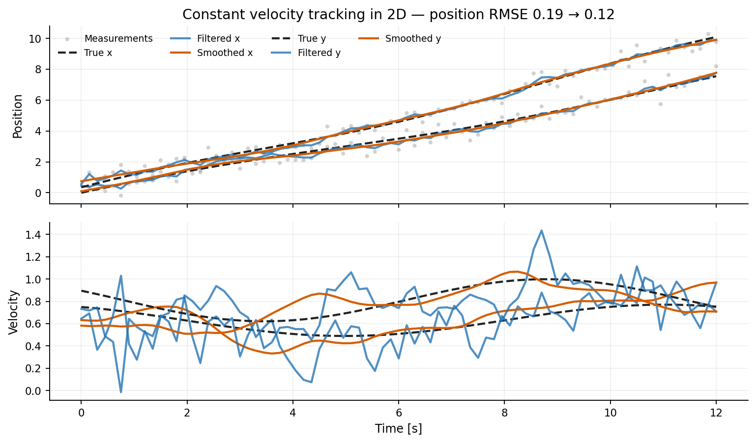
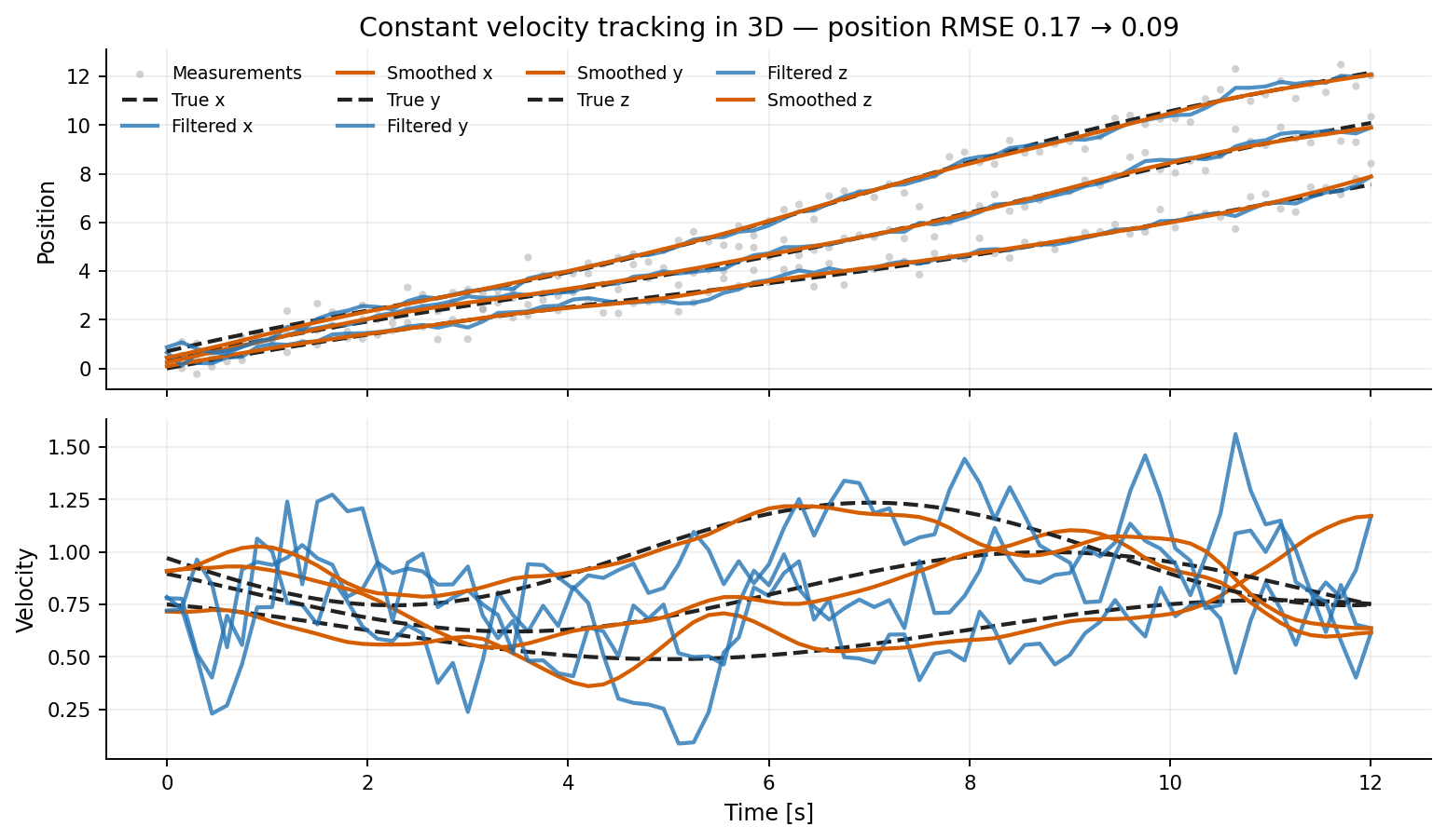
Constant-velocity tracking
For spatial dimension d, the state contains position and velocity:
x = [p, v]
The transition and position observation matrices are
F = [[I, dt I],
     [0,    I]]

H = [I, 0]
Process noise uses the discrete white-acceleration covariance
Q = q [[dt³/3, dt²/2],
       [dt²/2,    dt]] ⊗ I.
| 1D | 2D | 3D |
|---|---|---|
 |
 |
 |
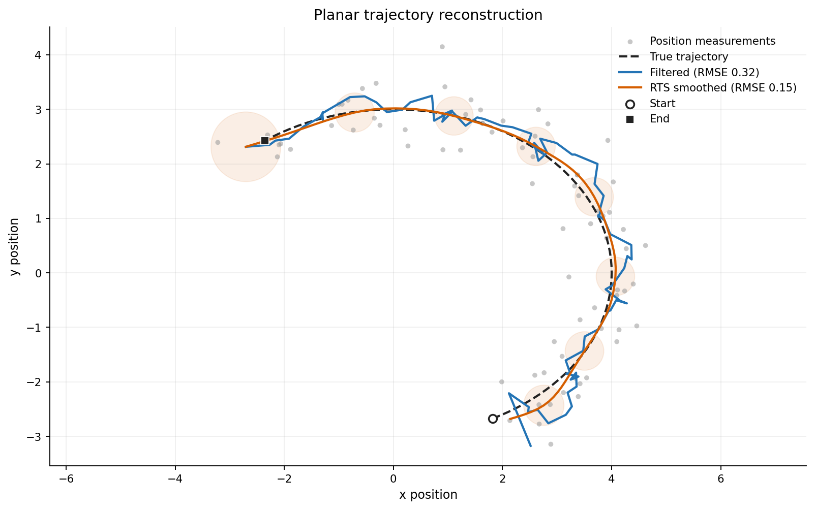
The same position-and-velocity state can reconstruct a curved planar trajectory. The ellipses below show selected 95% smoothed position-confidence regions.
Constant-acceleration tracking
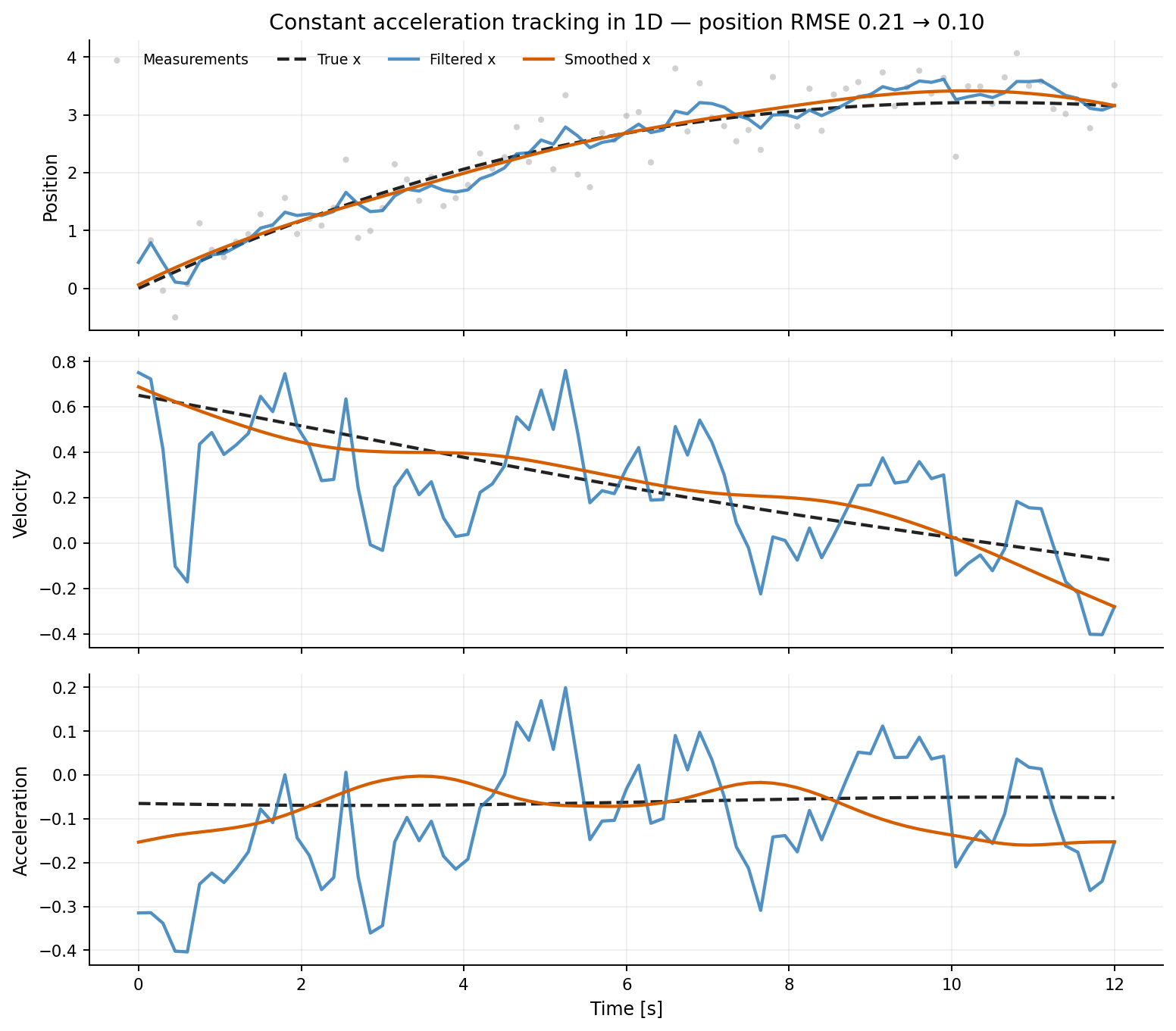
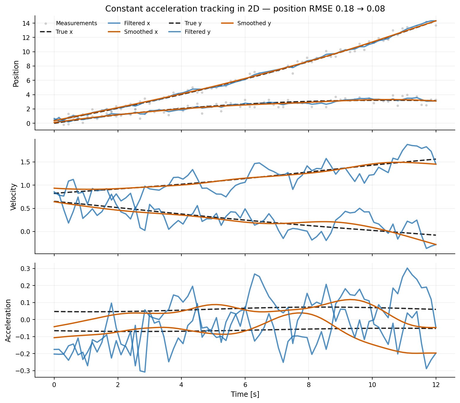
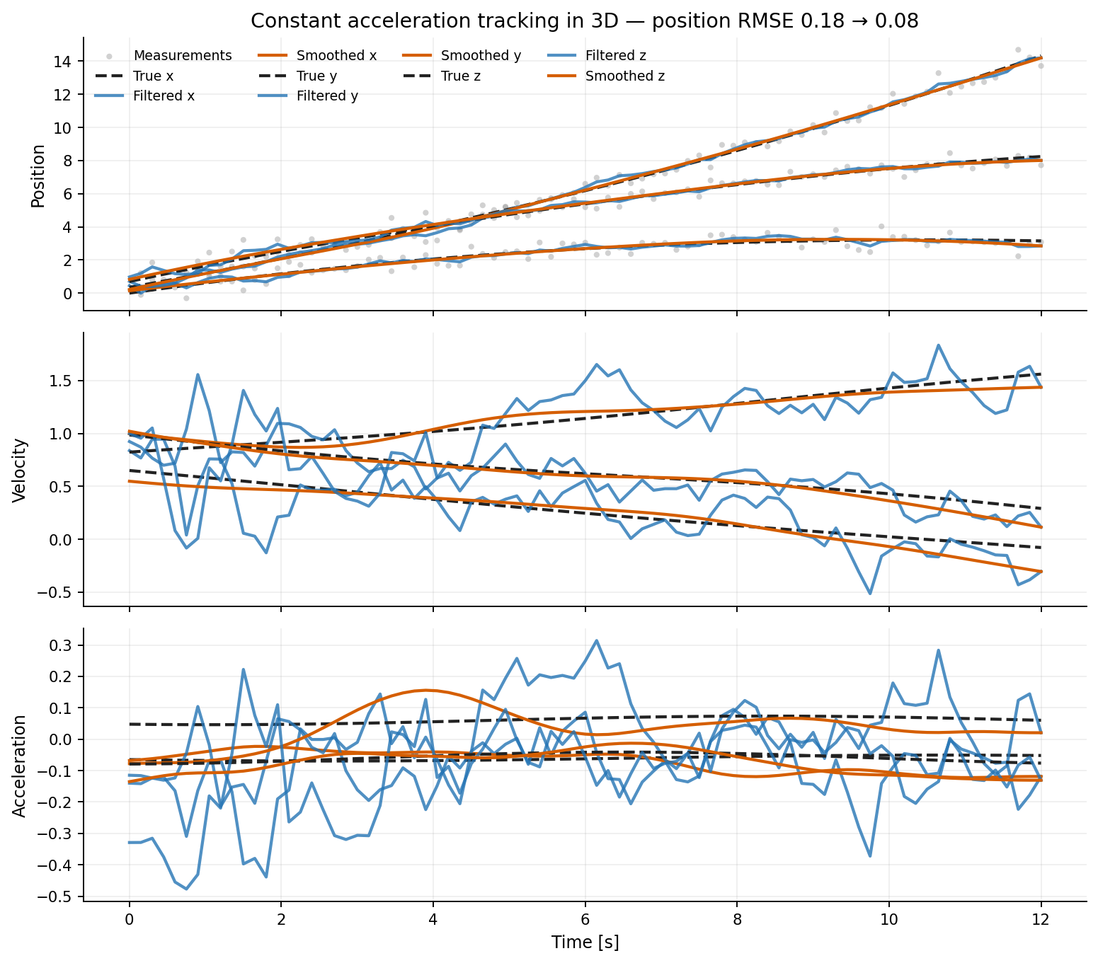
The state contains position, velocity, and acceleration:
x = [p, v, a]
Its transition is
F = [[I, dt I, ½ dt² I],
     [0,    I,     dt I],
     [0,    0,        I]].
Process noise uses the corresponding discrete white-jerk covariance. As in the velocity examples, noisy position is the only observed state component.
| 1D | 2D | 3D |
|---|---|---|
 |
 |
 |
The current transition-model API stores one fixed process covariance. These
examples therefore use fixed-cadence synchronous observations and construct
Q for that cadence.
Heading-coupled planar tracking
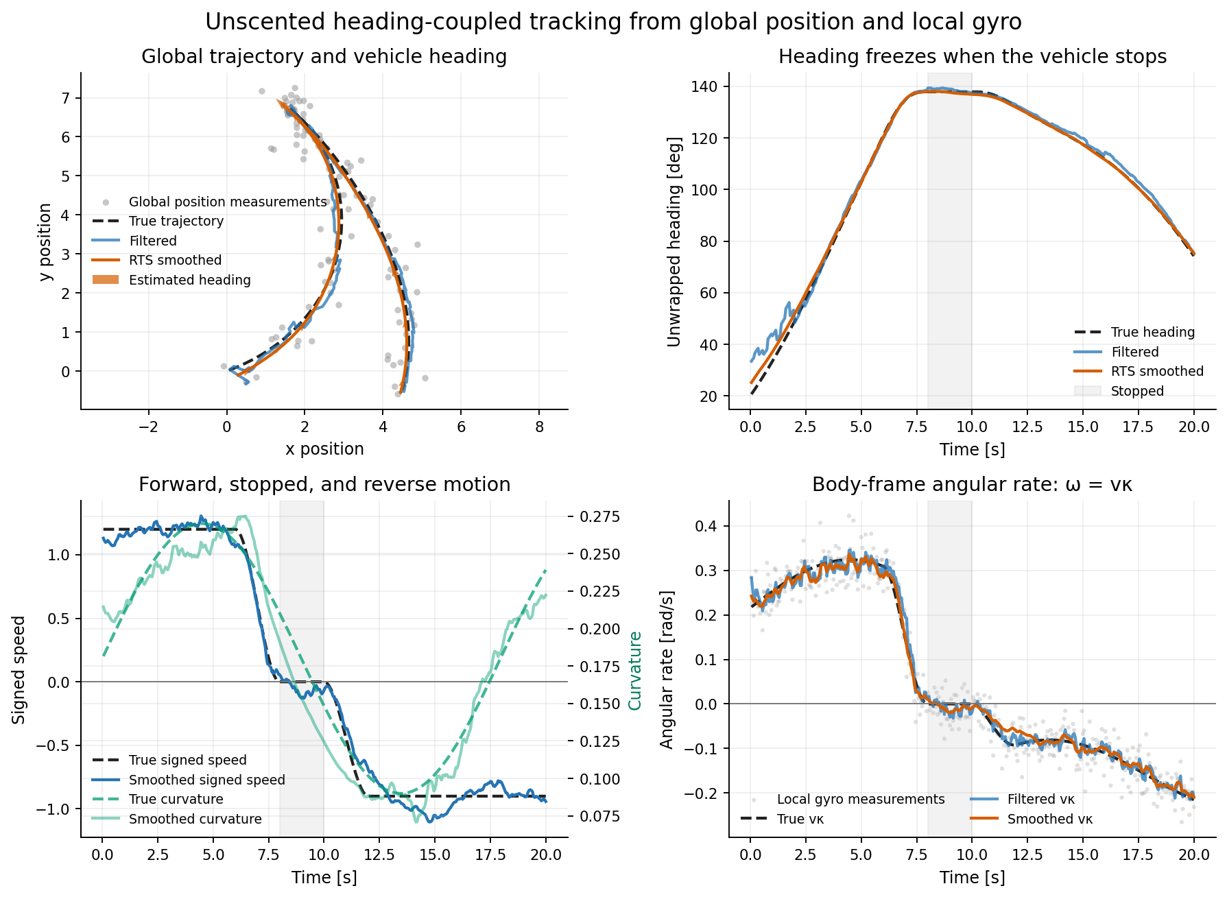
This example models a nonholonomic vehicle with state
x = [pₓ, pᵧ, ψ, v, κ],
where ψ is its unwrapped world heading, v is signed longitudinal speed,
and κ is signed curvature. Heading rate is coupled to motion:
ψ̇ = v κ.
The vehicle therefore cannot turn in place: both translation and heading rate
vanish when v = 0. Negative speed represents reversing and changes the sign
of the heading rate for fixed curvature. The discrete midpoint transition is
α = ψ + ½ dt v κ

pₓ' = pₓ + dt v cos(α)
pᵧ' = pᵧ + dt v sin(α)
ψ'  = ψ + dt v κ.
The filter asynchronously fuses noisy 5 Hz global position fixes with noisy 20 Hz body-frame angular-rate measurements:
z_position = [pₓ, pᵧ] + noise
z_gyro     = v κ + noise.
The deterministic trajectory drives forward, stops from 8–10 seconds, and then reverses. The default example uses unscented propagation; analytic Jacobians are also supplied and tested.
Nonlinear tracking and localization
Bearings-only target tracking
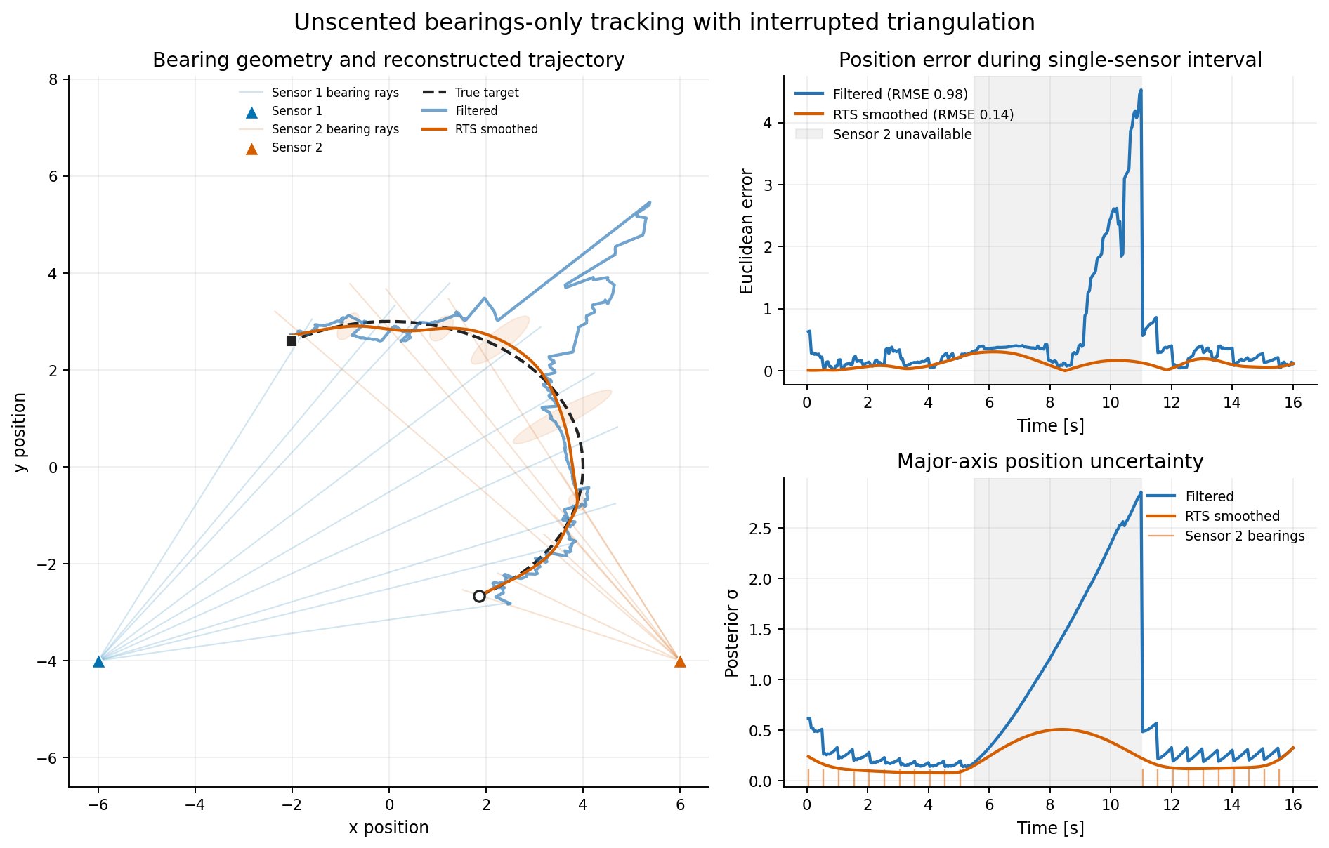
This example tracks a curved target without observing range or position directly. Two fixed sensors report noisy world-frame bearing unit vectors:
x = [pₓ, pᵧ, vₓ, vᵧ]

hᵢ(x) = (p - sᵢ) / ‖p - sᵢ‖,
where sᵢ is the position of sensor i. Encoding bearing as
[cos(bearing), sin(bearing)] avoids a discontinuous scalar residual at
±π. The observation remains strongly nonlinear and supplies no information
in the instantaneous line-of-sight direction.
Sensor 1 reports at 10 Hz. Sensor 2 reports at 2 Hz but is unavailable from 5.5–11 seconds. During that interval, range is only weakly observable from target motion, so the filtered uncertainty grows along the remaining bearing geometry. When sensor 2 returns, triangulation rapidly reduces it. The RTS smoother also uses those later measurements to reconstruct the dropout.
Radar + camera target fusion
This example tracks a maneuvering 2-D target with two complementary sensors.
The camera reports high-rate bearing as a unit vector,
u_cam = (p - c) / ||p - c||,
so it strongly constrains direction but provides no instantaneous range.
The radar reports lower-rate range and radial velocity,
rho     = ||p - r||
rho_dot = (p - r) . v / rho,
which strongly constrains radial position and motion but provides no bearing.
The target state is
x = [p_x, p_y, v_x, v_y].
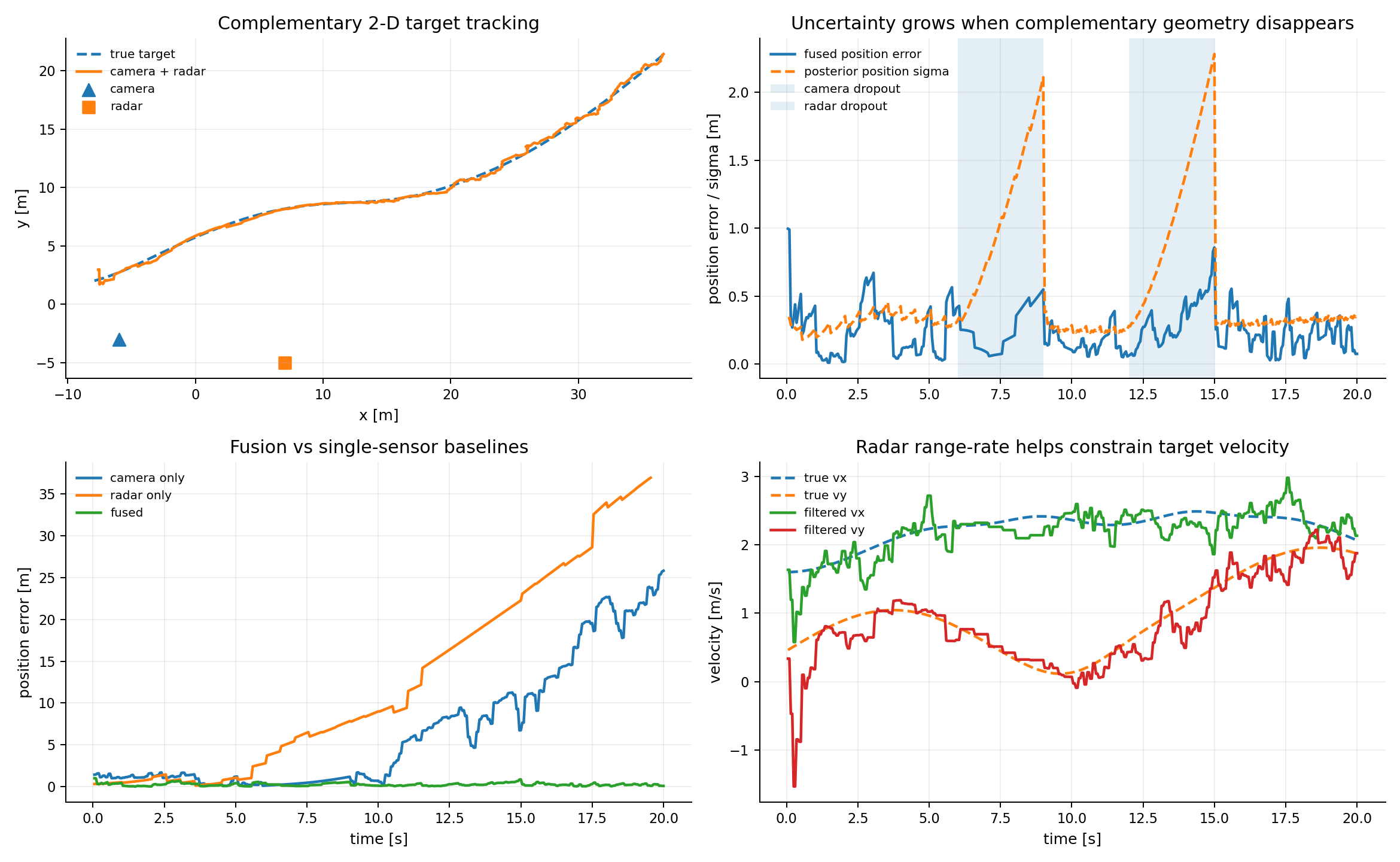
The example includes a camera dropout and a separate radar dropout. During camera loss, tangential uncertainty grows; during radar loss, range uncertainty grows. When both sensors are available, their complementary geometry keeps the track tight.
Camera-only and radar-only baselines use exactly the same prior and synthetic trajectory, making the improvement from fusion explicit. RTS smoothing then uses measurements after each dropout to reconstruct the missing interval more accurately.
TDOA emitter localization and clock calibration
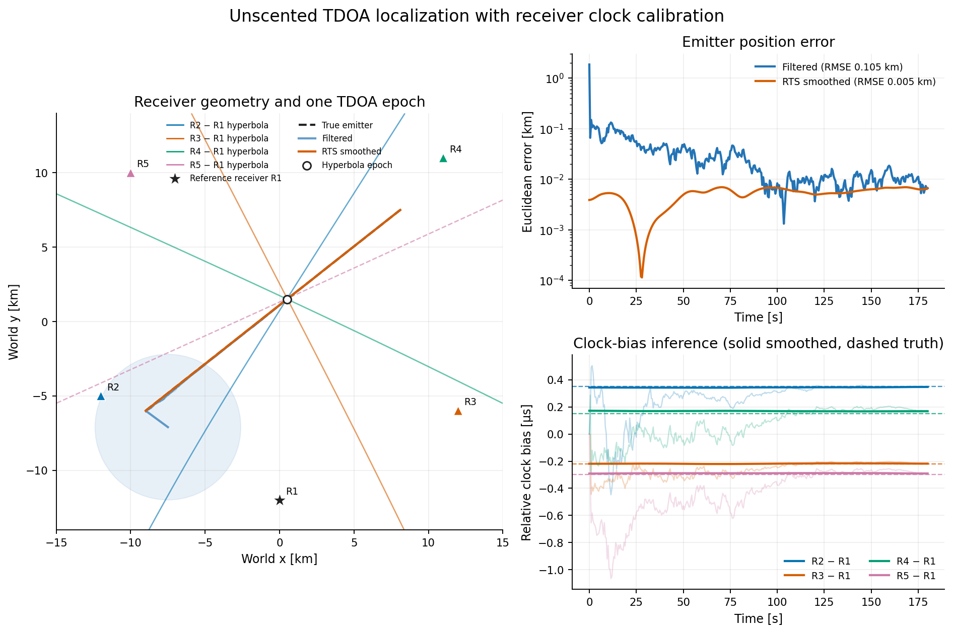
Five radio receivers localize a moving emitter without knowing when any pulse was transmitted. Subtracting the reference receiver's arrival time cancels the unknown emission time:
Δtᵢ₁ = (‖p - sᵢ‖ - ‖p - s₁‖) / c + bᵢ.
Here sᵢ is receiver position, c is the speed of light, and bᵢ is the
unknown clock offset of receiver i relative to receiver 1. The augmented
state
x = [pₓ, pᵧ, vₓ, vᵧ, b₂, b₃, b₄, b₅]
therefore estimates the trajectory and calibrates four clocks at once. Each TDOA constrains position to a hyperbola whose foci are the corresponding receiver pair. Their changing intersections, combined with the motion model, separate position from fixed clock bias.
All TDOAs share the same noisy reference timestamp, so their measurement noise is correlated. The example constructs the complete covariance matrix rather than treating the four differences as independent. Both Jacobian and unscented filtering paths are implemented and tested.
Doppler-only acoustic localization
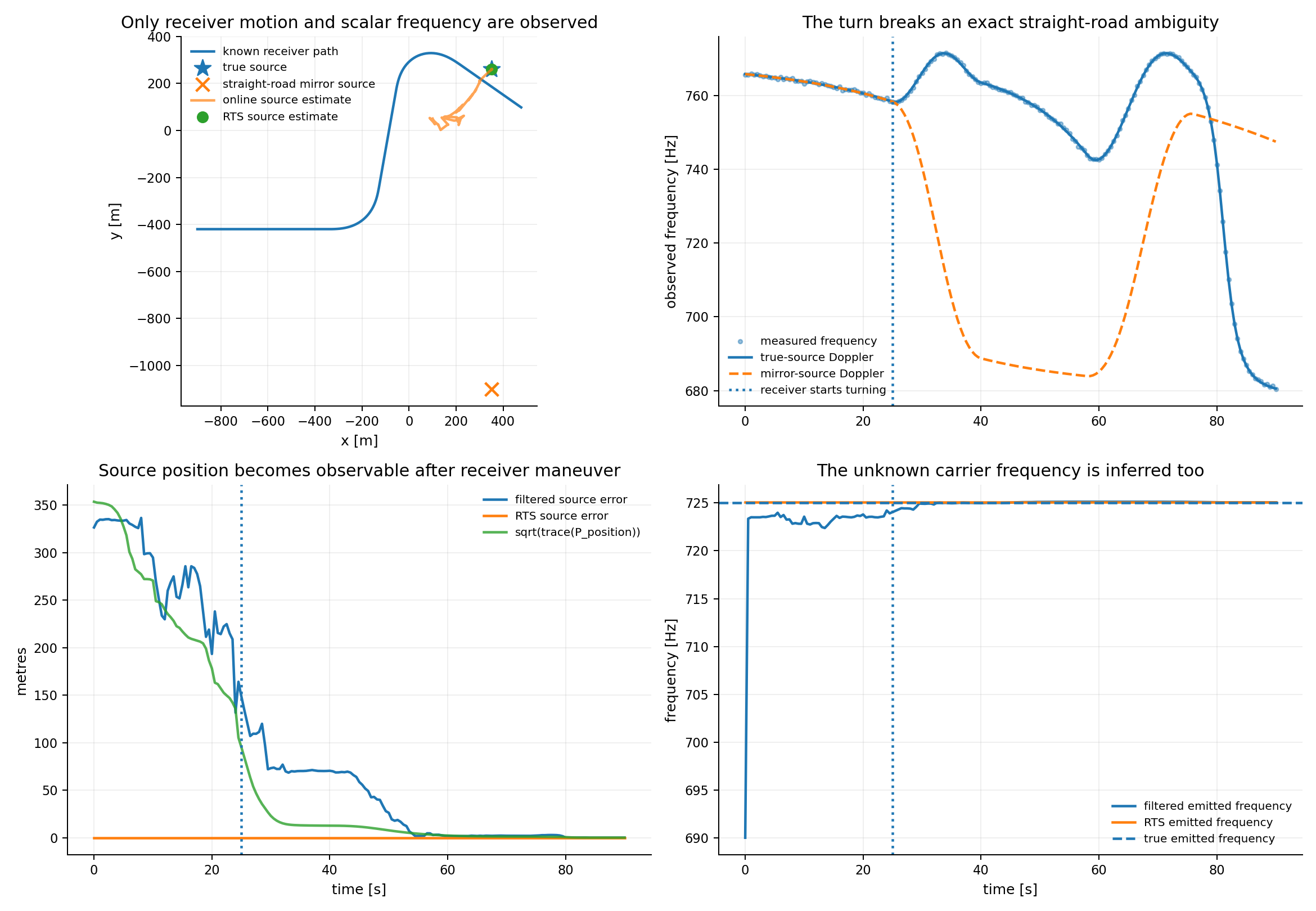
A moving receiver observes only apparent frequency from a stationary source whose emitted frequency is also unknown. Straight-line motion retains a mirror ambiguity; turning breaks it, and RTS smoothing reconstructs the earlier source location.
Ballistic radar tracking and drag inference
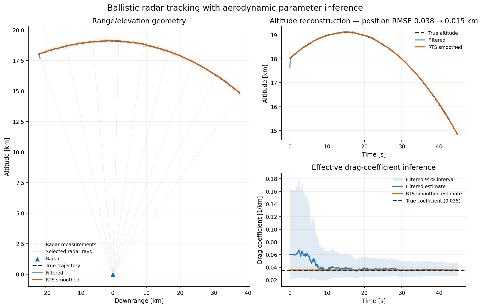
This example tracks a ballistic object in a two-dimensional exponential atmosphere while jointly estimating an unknown effective drag coefficient. The augmented state is
x = [rₓ, h, vₓ, vₕ, log(c_d)].
Using log drag keeps the inferred coefficient positive. Gravity and aerodynamic deceleration follow
ρ(h) / ρ₀ = exp(-h / H)
v̇ = [0, -g] - c_d exp(-h / H) ‖v‖ v.
A ground radar observes noisy slant range and elevation, but neither velocity nor drag directly:
z = [√(rₓ² + h²), atan2(h, rₓ)] + noise.
The coefficient becomes observable through accumulated curvature and deceleration. RTS smoothing uses the complete radar arc to improve the early trajectory and parameter estimate.
Navigation and mapping
Local/global vehicle fusion
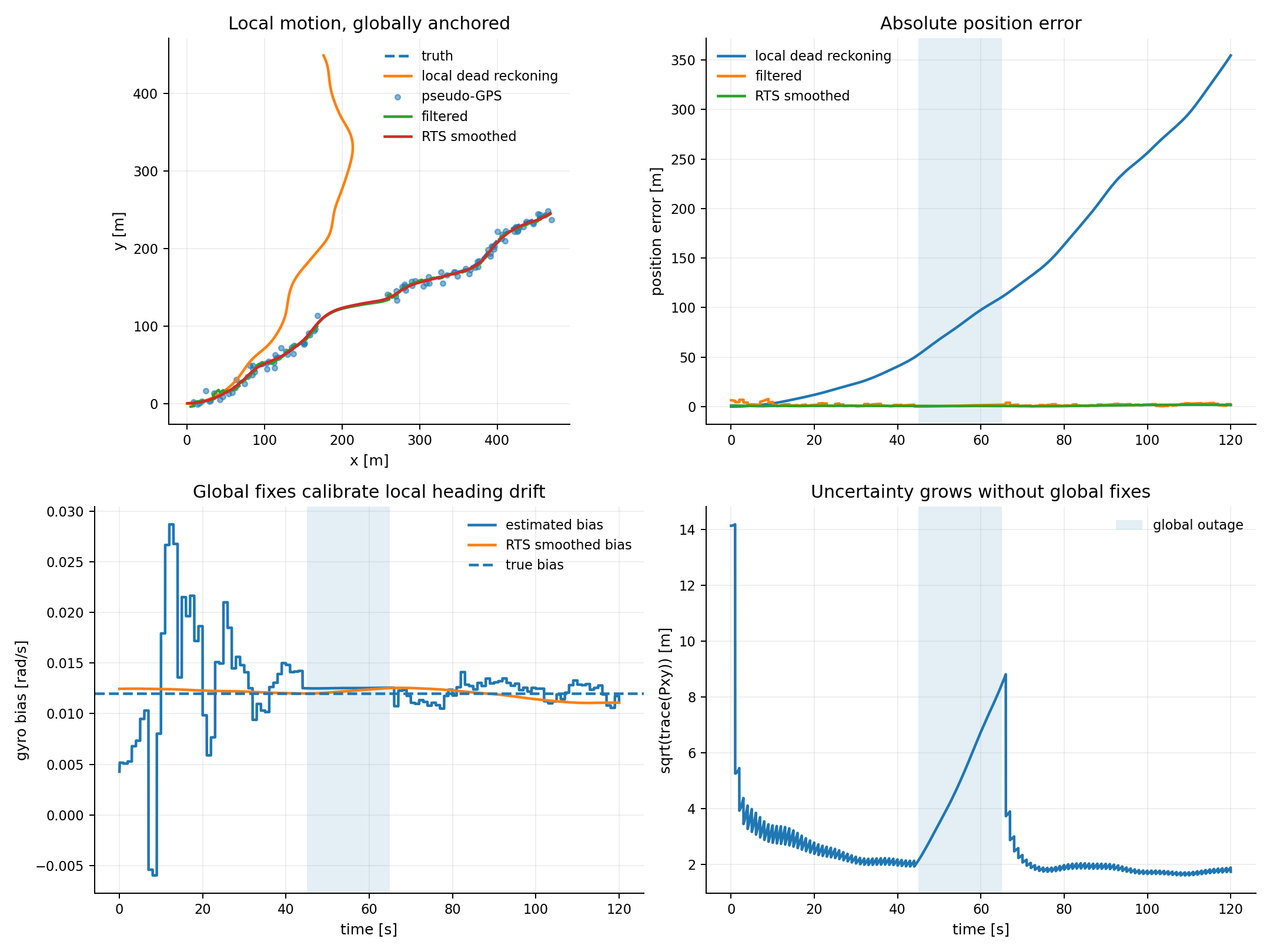
High-rate speed and gyro measurements propagate a planar trajectory between slow global position fixes. A long global-sensor outage demonstrates dead reckoning, gyro-bias inference, uncertainty growth, reacquisition, and RTS reconstruction.
Black-box INS and GPS fusion
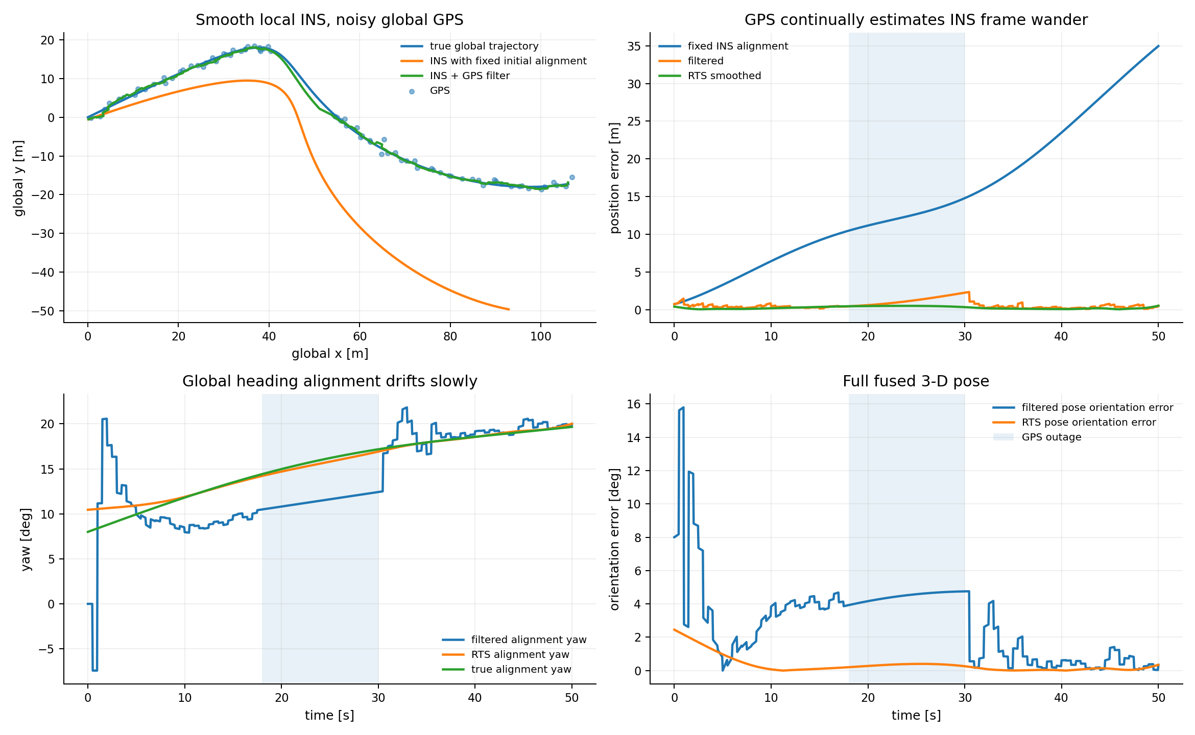
Rather than re-integrating IMU samples, this example aligns an existing smooth local 6-DoF INS trajectory to sparse global GPS positions by estimating a slowly drifting translation and yaw transform. A 12-second GPS outage makes the difference between online filtering and offline smoothing explicit.
Sun-aided island navigation
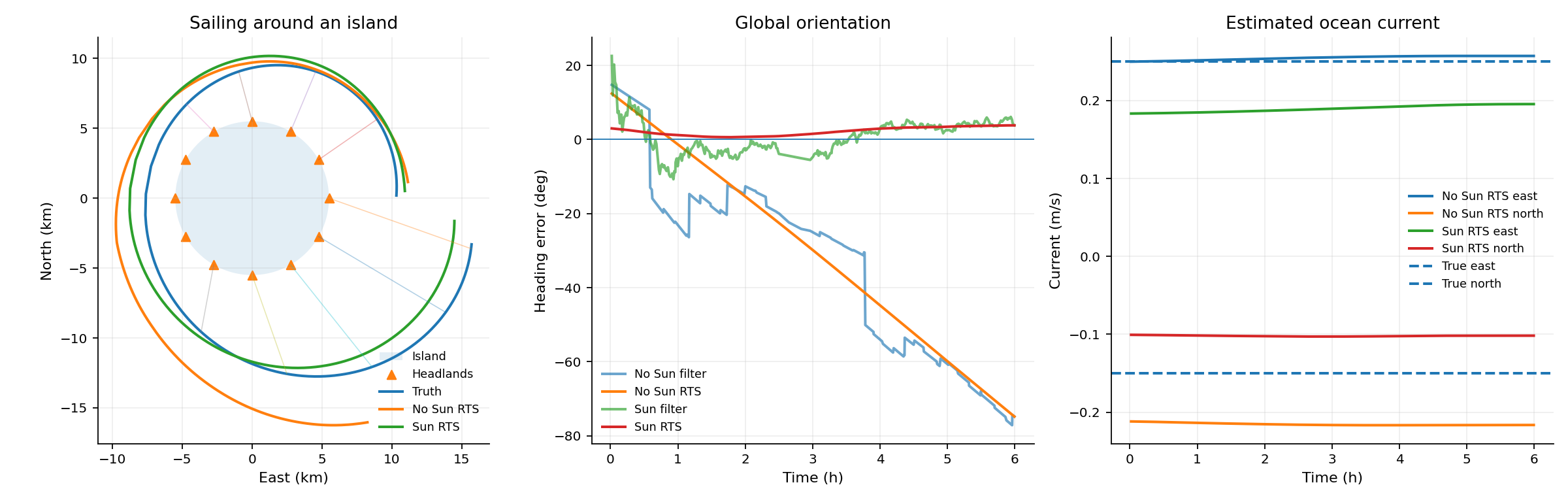
A sailing vessel fuses a noisy speed log, occasional human range/bearing estimates to a charted headland, and body-frame Sun directions. The filter jointly estimates position, heading, turn rate, and a steady ocean current; a no-Sun ablation exposes the value of the global orientation cue.
Boat current and compass-bias inference
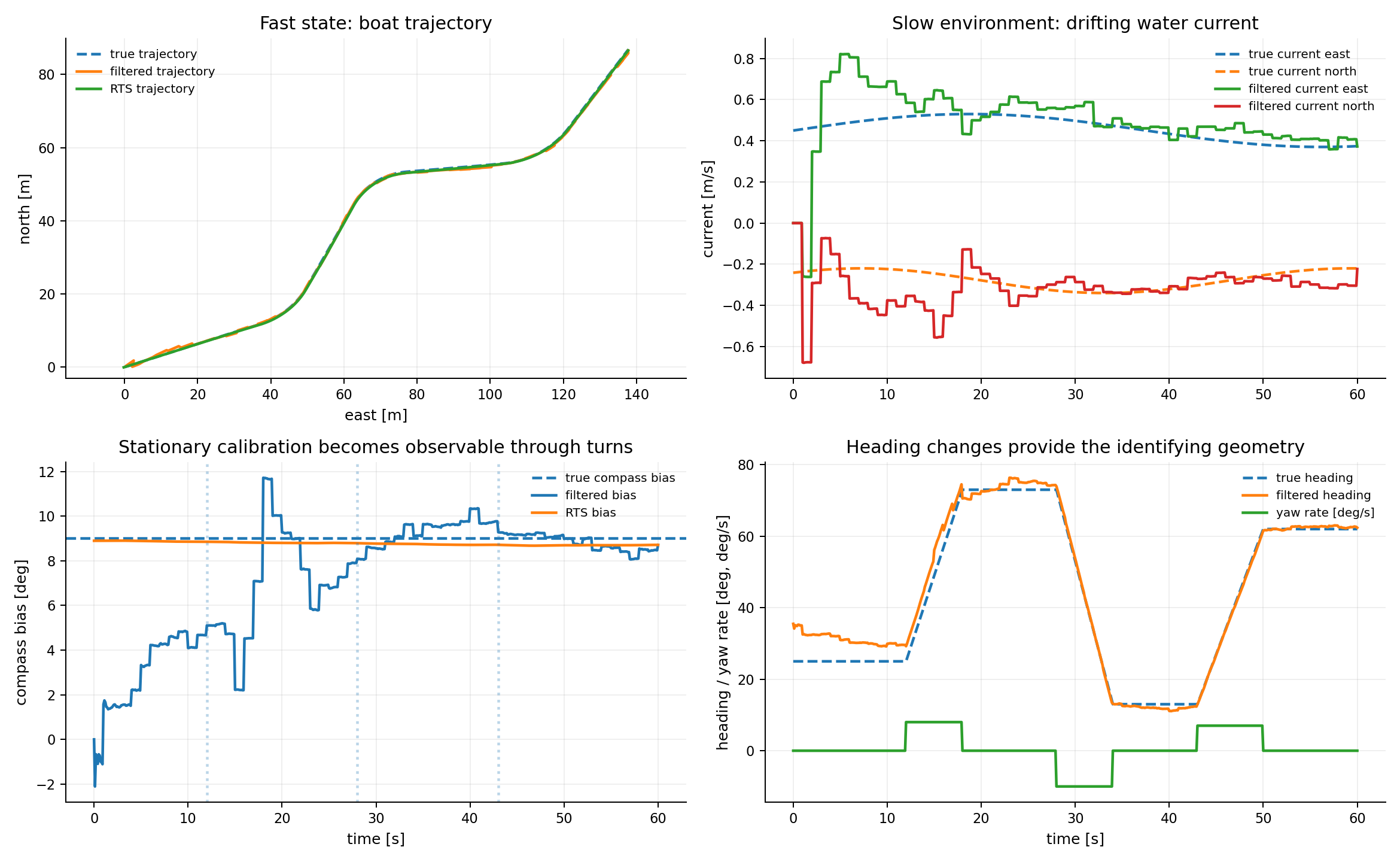
GPS, speed-through-water, yaw-rate, and magnetic-heading observations jointly recover boat motion, a slowly drifting water-current vector, and a stationary compass bias. Direction changes provide the geometry that separates current from calibration error.
Known-correspondence landmark SLAM
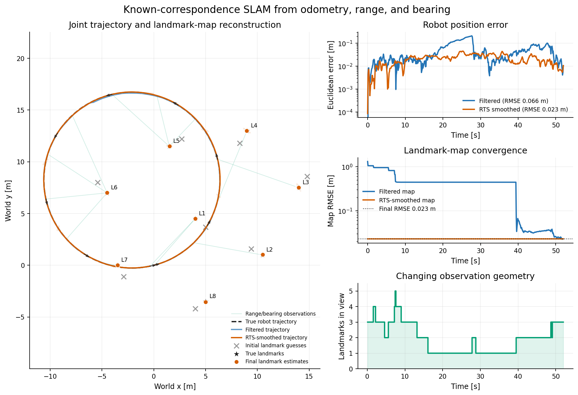
This example jointly estimates a planar robot trajectory and the coordinates of eight initially uncertain landmarks. Each observation carries a known landmark identity, so the state has fixed dimension:
x = [pₓ, pᵧ, ψ, v, ω, ℓ₁ₓ, ℓ₁ᵧ, …, ℓ₈ₓ, ℓ₈ᵧ].
The robot follows a heading-coupled coordinated-motion model. Wheel odometry
measures forward speed and yaw rate, while visible landmarks provide noisy
range and bearing. As in the bearings-only example, bearing is represented by
a local-frame unit vector to avoid a discontinuous residual at ±π:
ρᵢ = ‖ℓᵢ - p‖
uᵢ = R(-ψ) (ℓᵢ - p) / ρᵢ.
SLAM determines geometry only up to an arbitrary global translation and rotation. The example therefore uses a tight prior on the initial robot pose to define the world frame, while landmark priors begin more than a metre from their true positions. The robot completes a loop through the map, repeatedly changing which landmarks fall inside the sensor range and field of view. Reobserving early landmarks closes the loop and sharpens both the trajectory and map.
The default run uses analytic Jacobians, as in classical EKF-SLAM. Unscented filtering and smoothing are also supported and covered by the tests.
Aircraft bank inference
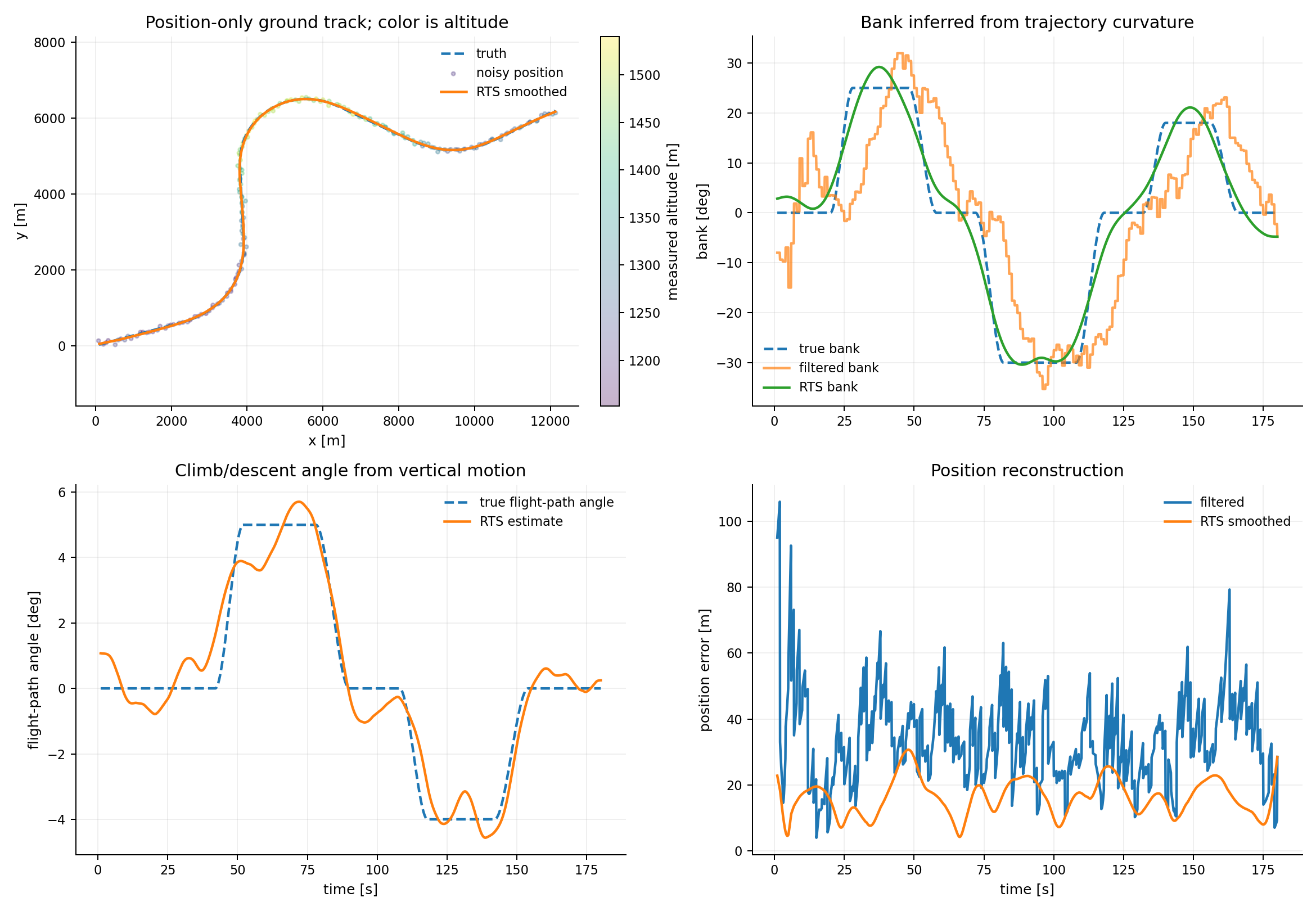
Only noisy global position is measured. A coordinated-flight model couples horizontal curvature to bank angle and vertical motion to flight-path angle, making both latent maneuver variables observable from the track.
Space and orbital estimation
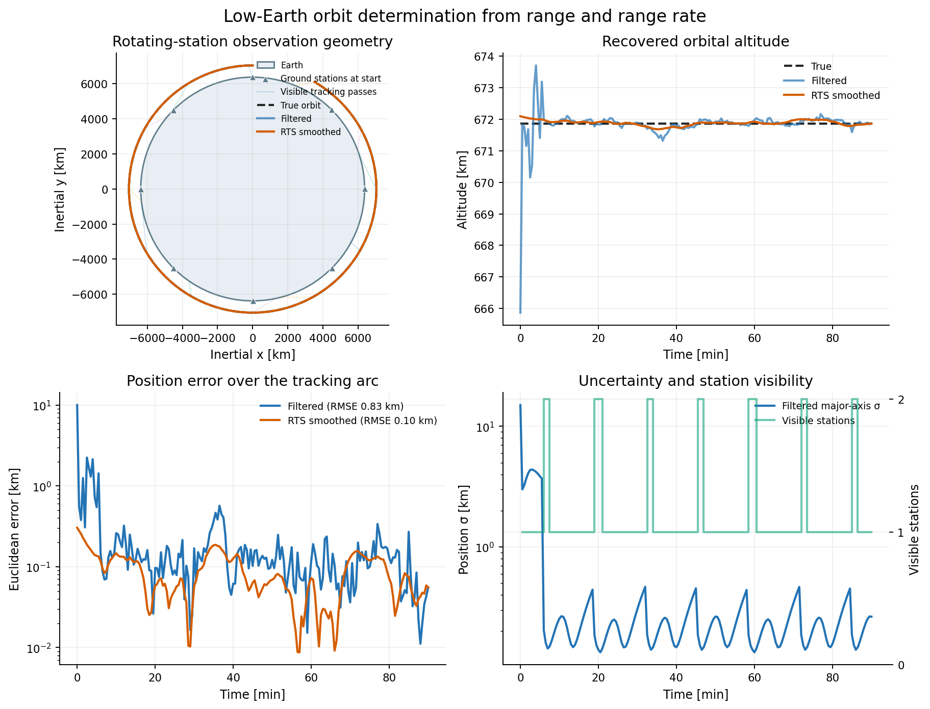
Orbit determination from rotating ground stations
The orbit example propagates a planar low-Earth satellite under two-body gravity in an inertial frame:
x = [r, v]
ṙ = v
v̇ = -μ r / ‖r‖³.
Eight equatorial stations rotate with Earth. A station contributes an observation only while the satellite is above its local horizon. Each visible station measures nonlinear range and range rate:
ρ  = ‖r - sᵢ(t)‖
ρ̇ = (r - sᵢ(t)) · (v - ṡᵢ(t)) / ρ.
The unscented filter recovers position and velocity from the changing station geometry, while the RTS pass reconstructs a consistent orbit over the full 90-minute tracking arc.
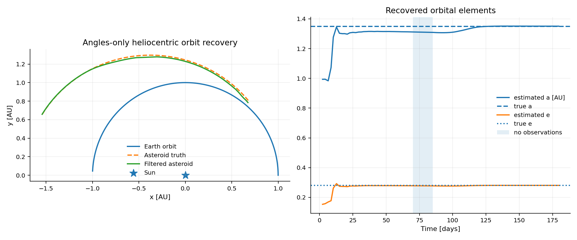
Angles-only asteroid orbit determination
A moving Earth observer measures only telescope line-of-sight directions. The changing baseline and solar two-body dynamics recover the asteroid's heliocentric position and velocity without direct range observations.
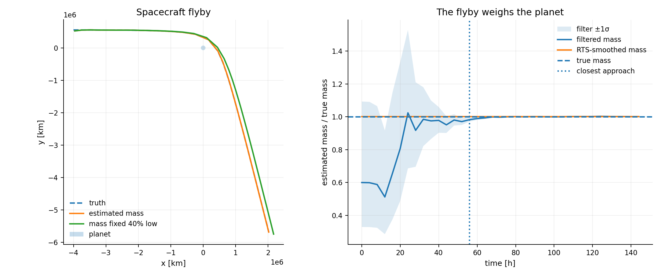
Planet mass from a spacecraft flyby
The spacecraft state includes log(mu), allowing gravitational bending during
a close flyby to identify a planet's mass while position and velocity are
tracked from noisy navigation fixes.
Rigid-body and inertial estimation
Rigid-body state and dynamics
The rigid-body state is
x = [p, v, ϕ, ω],
where p and v are world-frame center position and velocity, ω is
body-frame angular velocity, and ϕ ∈ R³ is a rotation bivector/vector. Its
equivalent representations are
R = Exp([ϕ]×)
q = Exp(½ [0, ϕ])
ϕ = 2 vec(Log(q)).
Translation follows constant velocity. Rotation follows the torque-free Euler
equation for a body with inertia matrix I:
I ω̇ + ω × (I ω) = 0.
Angular velocity is integrated with RK4. Attitude is advanced by composition on SO(3):
R_next = R Exp([dt ω_mid]×).
The state is then returned to bivector coordinates with Log(R_next). The
examples remain inside one principal-log chart and do not cross the π branch
boundary. BayesFilter does not yet provide manifold-aware Gaussian means or
retractions, so this chart restriction is intentional.
World-space point observations
The body carries four labeled canonical points:
c₀ = 0, c₁ = 0.75 e₁, c₂ = 0.75 e₂, c₃ = 0.75 e₃.
Their predicted world locations are
hᵢ(x) = p + R(ϕ)cᵢ.
The origin marker observes translation directly. Subtracting it from the other marker positions recovers scaled columns of the rotation matrix. The filter residual therefore lives in ordinary Cartesian point space; it never subtracts quaternions or rotation vectors directly.
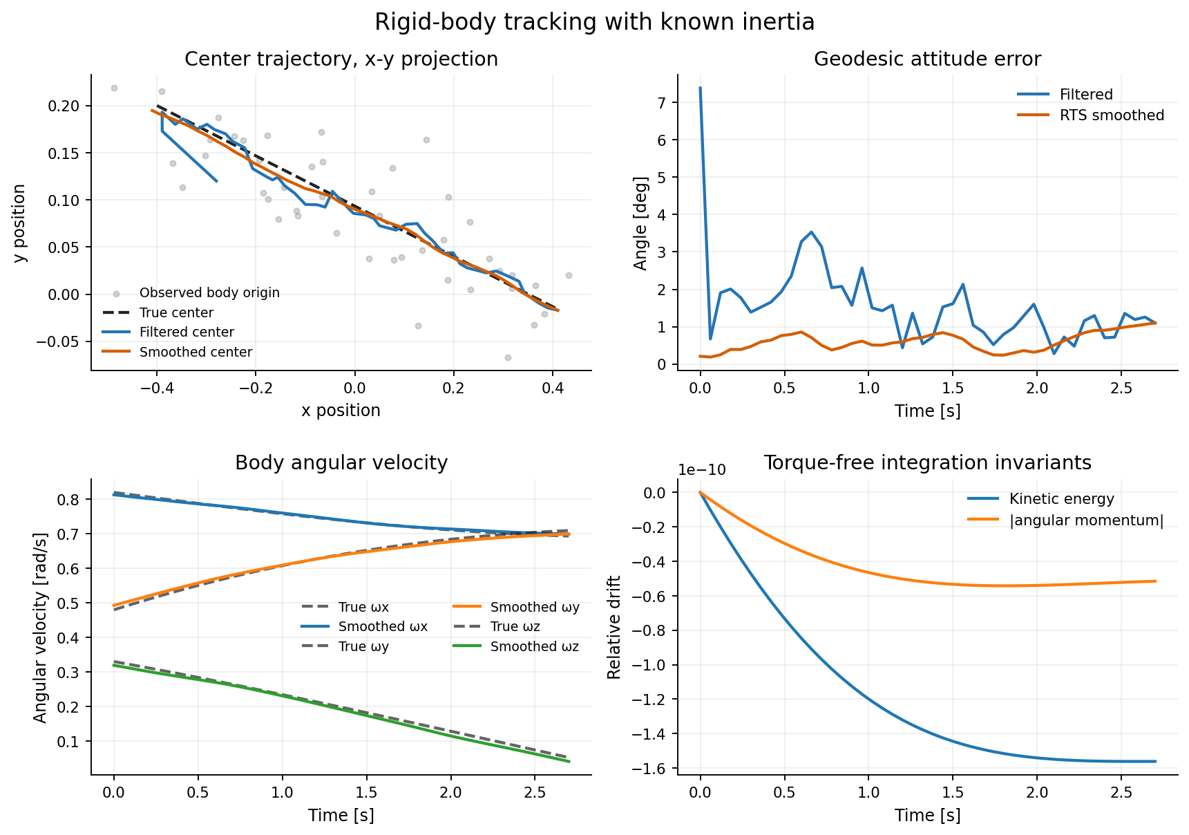
Known fixed inertia
The known-inertia example uses diag(1.0, 1.4, 1.8) and the unscented filter
and smoother. Its figure shows position tracking, geodesic attitude error,
body angular velocity, and numerical conservation of torque-free invariants.
Inferring inertia ratios in the state
Torque-free angular motion is unchanged if every principal moment is scaled
by the same constant. Absolute inertia scale is therefore unobservable from
these measurements. The augmented example fixes I₁ = 1 and estimates the
two identifiable log ratios
η₂ = log(I₂ / I₁), η₃ = log(I₃ / I₁).
Exponentiation keeps the inferred ratios positive. The parameters have tiny process noise and are inferred indirectly from the observed world-space point trajectories—there are no direct angular-velocity or inertia measurements. The default run uses 100 point-observation sets over four seconds, making both the ratio convergence and posterior-uncertainty contraction visible.
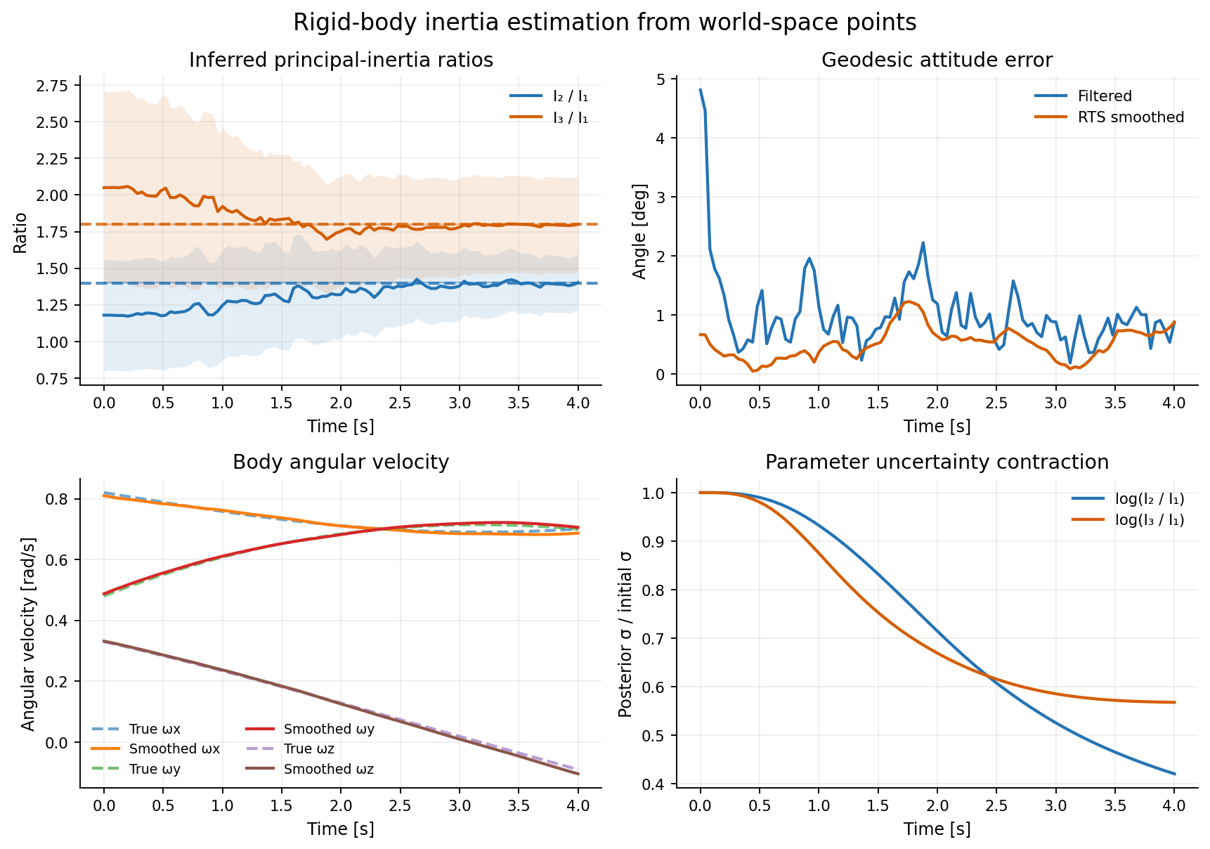
To identify absolute inertia scale, an example would need a known applied torque or another measurement that supplies scale information.
Gravity vector from raw IMU data
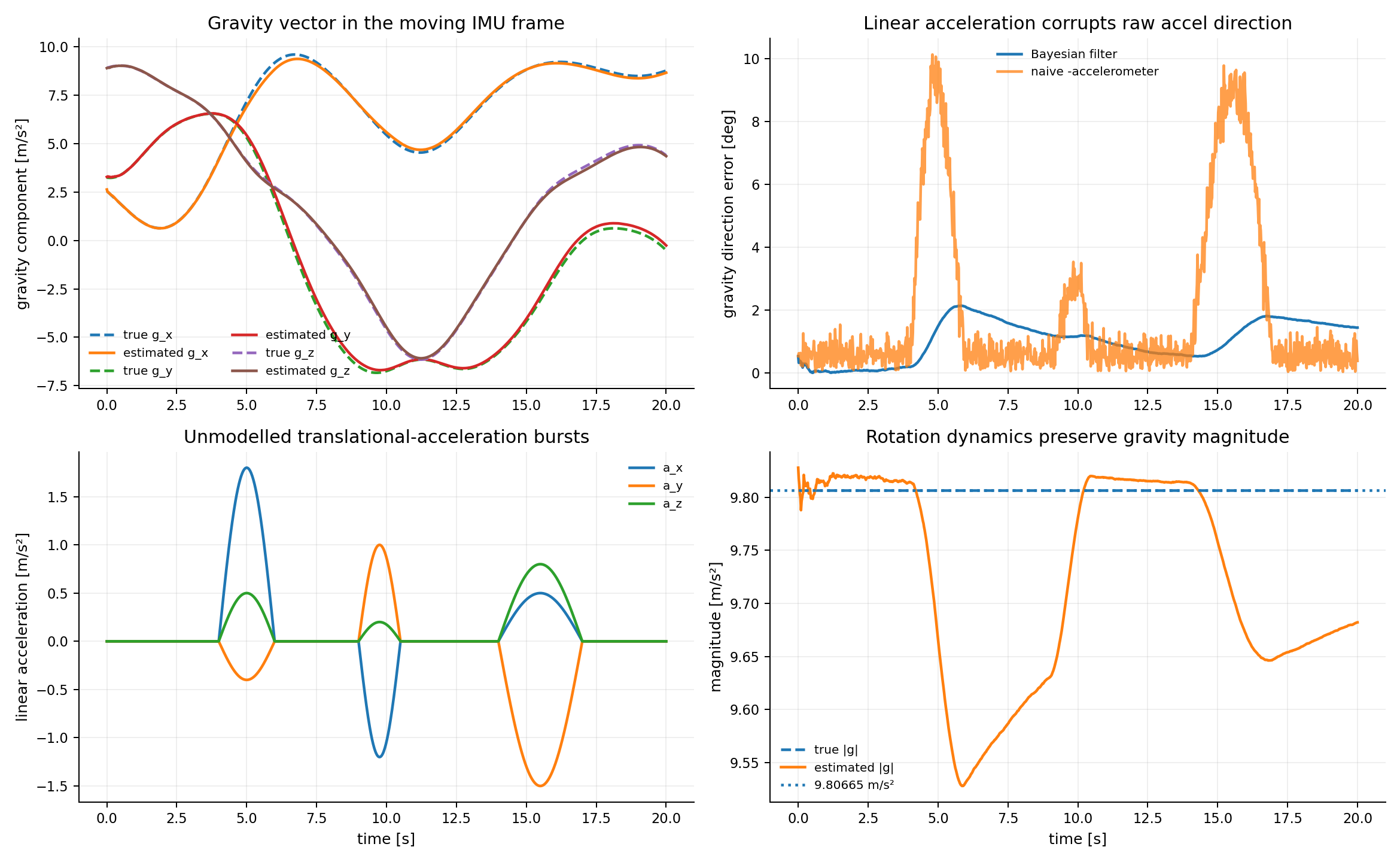
This example estimates gravity expressed in the moving IMU frame directly from raw gyroscope and accelerometer measurements. The state is
x = [g_x, g_y, g_z, ω_x, ω_y, ω_z].
A world-fixed gravity vector evolves in body coordinates according to
g_dot = -ω × g.
The gyro therefore propagates the gravity direction through rotations, while
the accelerometer supplies a long-term specific-force cue. Several deliberate
linear-acceleration bursts make the raw accelerometer direction temporarily
wrong; the fused estimate remains much less disturbed than simply using
g = -a.
Phone gyrocompassing from hand reorientation
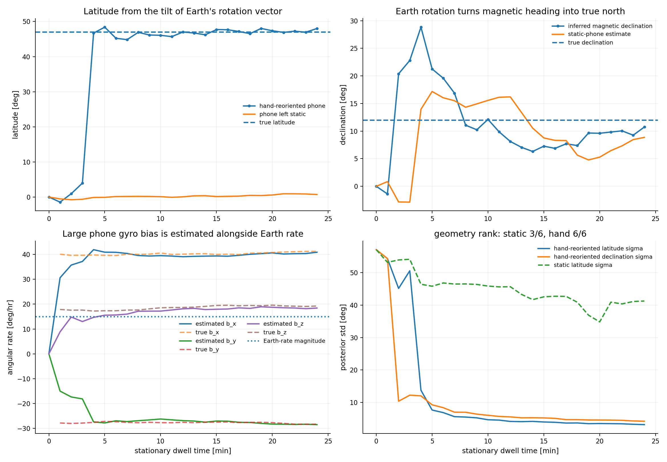
A consumer phone is held still, moved by hand to an arbitrary new orientation, and held still again. The hand rotation rate and exact stop angle are never provided. During each stationary dwell, gravity and the calibrated magnetic field reconstruct the phone pose relative to magnetic north; the averaged gyro then observes
z_g = R_i Ω_E + b_g + noise.
The six-state filter estimates the Earth-rate vector in the magnetic local frame together with the slowly drifting phone-frame gyro bias:
x = [Ω_magnetic, b_g].
A static phone is rank-deficient because Earth rate and constant gyro bias cannot be separated. Diverse hand reorientations rotate the Earth vector while the sensor bias remains attached to the phone, making the calibration full rank. Latitude follows from the vertical component of the inferred Earth-rate vector, while the horizontal angle between magnetic north and the Earth-rate projection gives magnetic declination and therefore true north.
The synthetic gyro noise uses published Pixel 7 Pro MEMS measurements. The default experiment uses 24 one-minute stationary dwells and deliberately starts with a turn-on gyro bias larger than the 15 deg/hour Earth-rate signal.
Sensor and geometric calibration
Camera/gyro spatiotemporal calibration
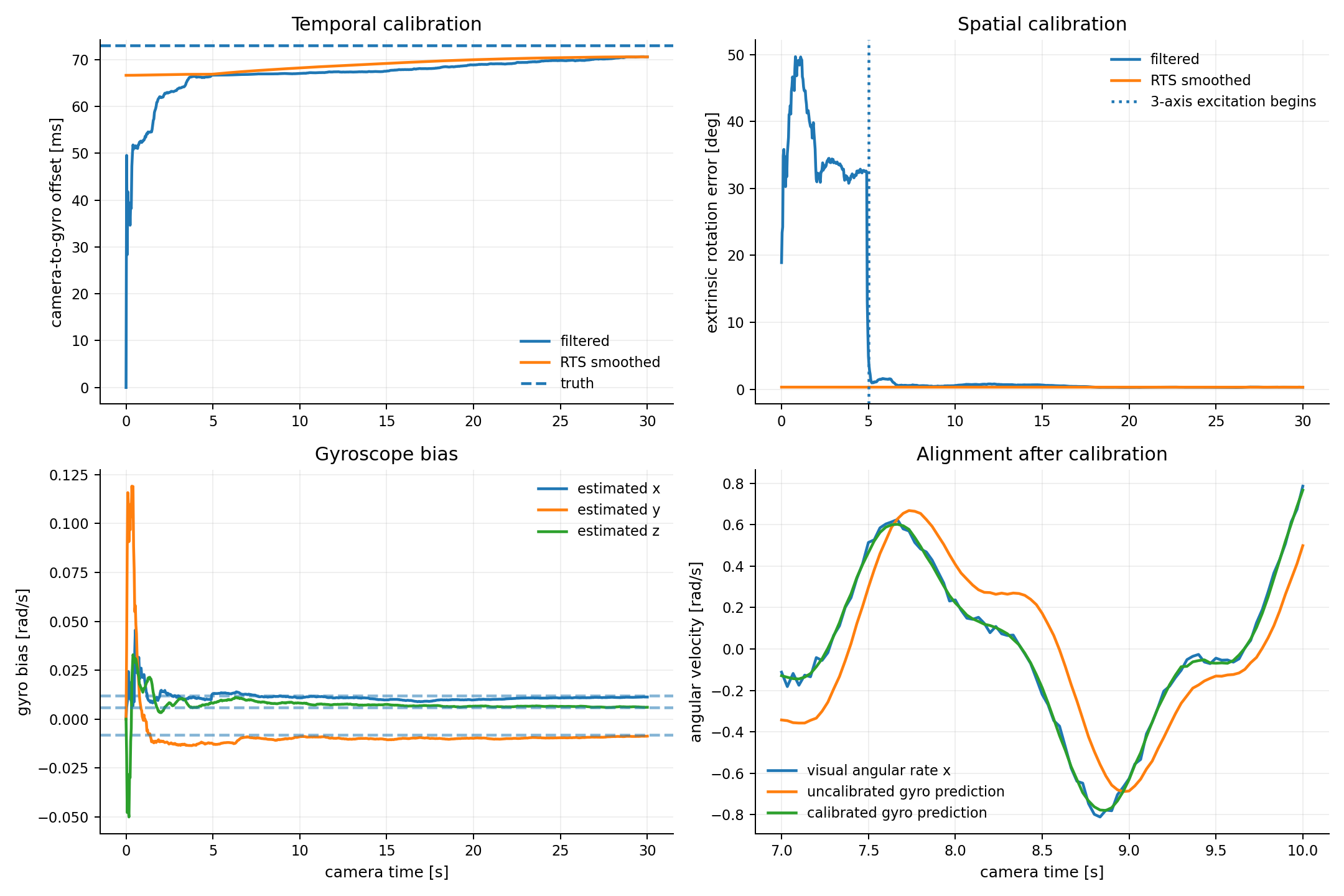
Asynchronous camera and gyroscope angular-velocity streams identify their relative rotation, clock offset, and gyro bias. Early single-axis motion is weakly observable; later three-axis excitation completes the calibration.
Wrist-camera hand-eye calibration
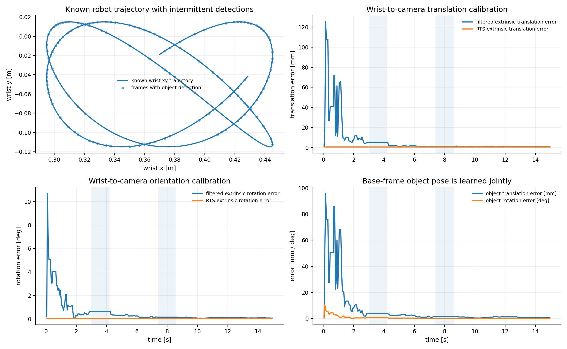
This example calibrates a wrist-mounted camera while a robot moves through a known 6-DoF Cartesian wrist trajectory and intermittently detects the pose of a fixed object on a table.
Using the transform convention ^A T_B for a transform from frame B into
frame A, each detection obeys
^B T_O = ^B T_W(t) ^W T_C ^C T_O(t).
The known quantity is the robot wrist pose ^B T_W(t). The camera detector,
whose intrinsics are assumed known upstream, produces the object pose
^C T_O(t) only on frames where the object is detected.
The filter jointly estimates
state = [t_WC, phi_WC, t_BO, phi_BO],
where ^W T_C is the desired wrist-to-camera extrinsic and ^B T_O is the
unknown but stationary object pose in the robot base frame. The object
therefore does not need to be surveyed independently.
Each 6-DoF detected object pose is used through a local SE(3) residual,
r = [t_pred - t_meas,
     Log(R_meas^T R_pred)].
This keeps translation and rotation in their natural detector noise scales and avoids both a global rotation-vector subtraction and an arbitrary synthetic lever arm.
The synthetic detector succeeds on only about 45% of frames and includes two longer gaps. Missing detections simply produce no observation; the stationary calibration state propagates with effectively zero process noise.
The nonlinear calibration is refined with three complete forward/backward passes:
UKF_1 -> RTS_1 -> UKF_2 -> RTS_2 -> UKF_3 -> RTS_3
After each RTS pass, the smoothed estimate at the beginning of the sequence is used as the mean of the next UKF prior. The original broad prior covariance is restored for every new forward pass, so the repeated optimization improves the nonlinear starting point without pretending that the same measurements are independent new information.
The default camera prior is intentionally generic and does not use the true extrinsic. The unknown base-frame object pose is bootstrapped from the first successful object detection using that same crude camera guess. An explicit zero-translation / identity-rotation camera start is also covered by the tests.
Multi-axis wrist rotation is important. Pure or nearly pure translation leaves parts of hand-eye calibration poorly observable, whereas the example's varied orientation trajectory separates camera translation, camera rotation, and the unknown base-frame object pose.
GNSS and IMU lever-arm calibration
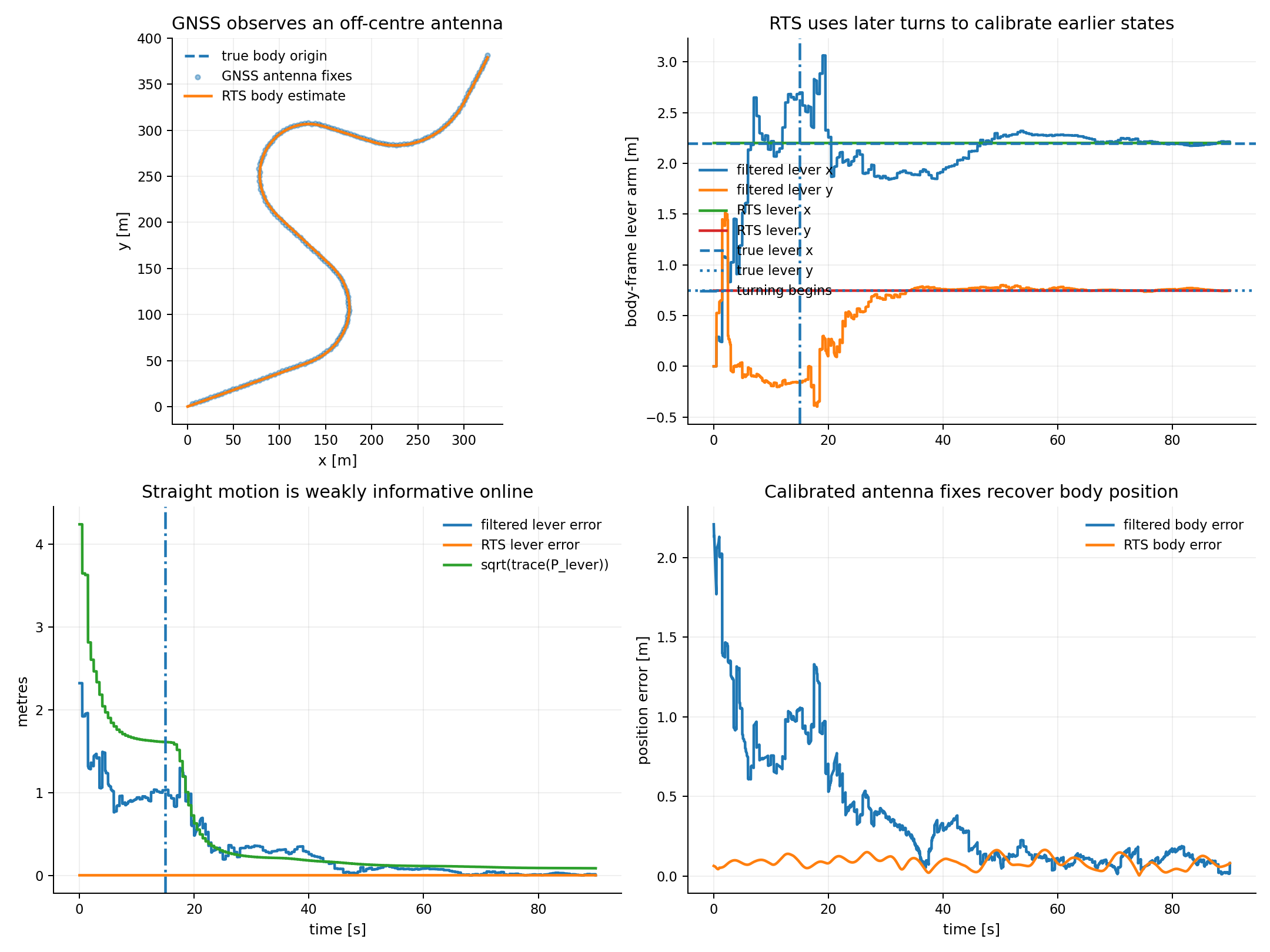
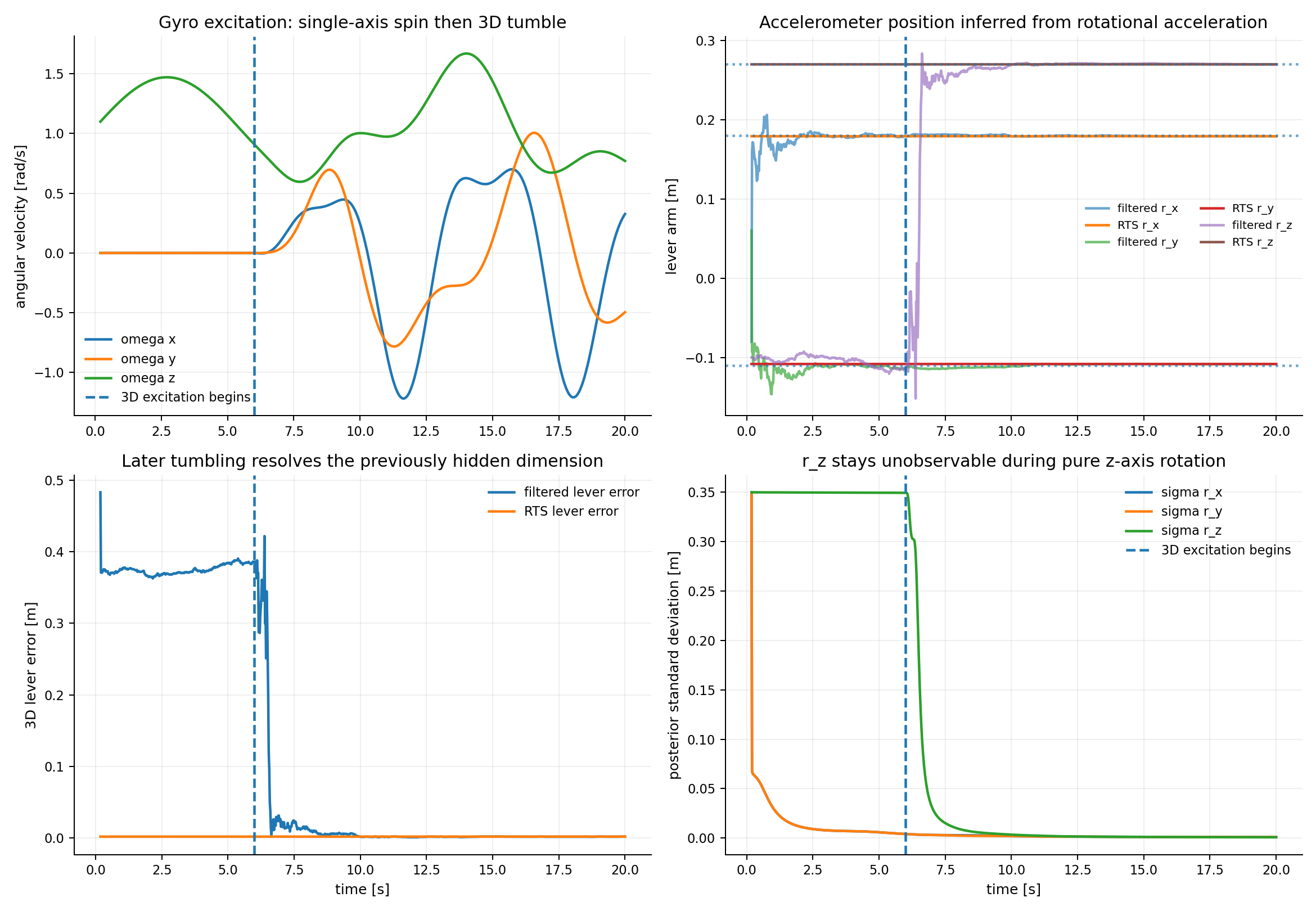
Vehicle turns rotate an unknown GNSS antenna offset into the world frame, separating it from body position. In the three-dimensional IMU example, angular and centripetal acceleration identify an accelerometer's mounting position and bias after multi-axis excitation.
| GNSS antenna lever arm | Accelerometer lever arm |
|---|---|
 |
 |
Wheel-radius and speedometer calibration
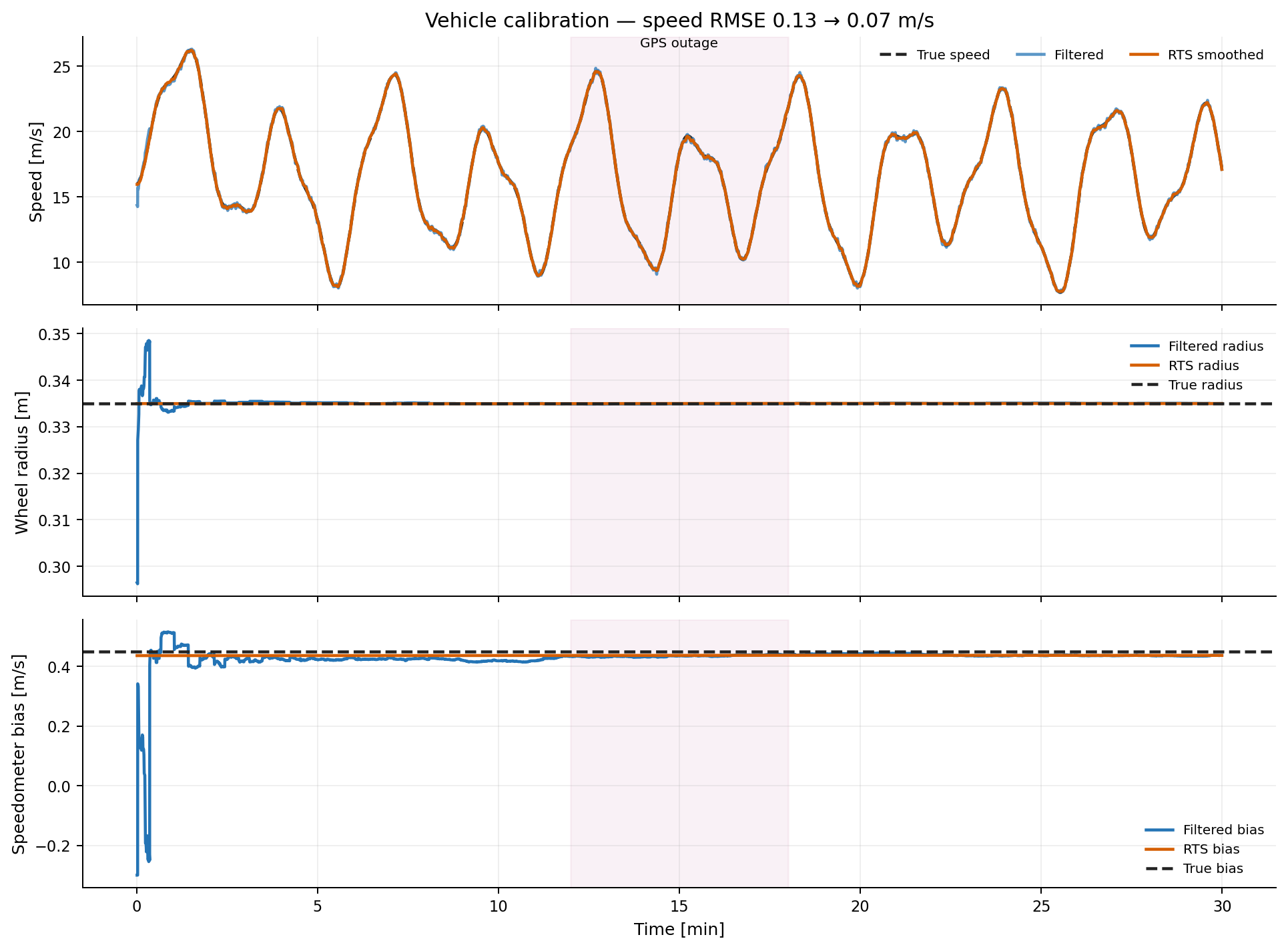
This example identifies effective wheel radius and dashboard-speed bias from wheel, speedometer, and sparse GPS measurements through a six-minute GPS outage.
Physical parameter inference
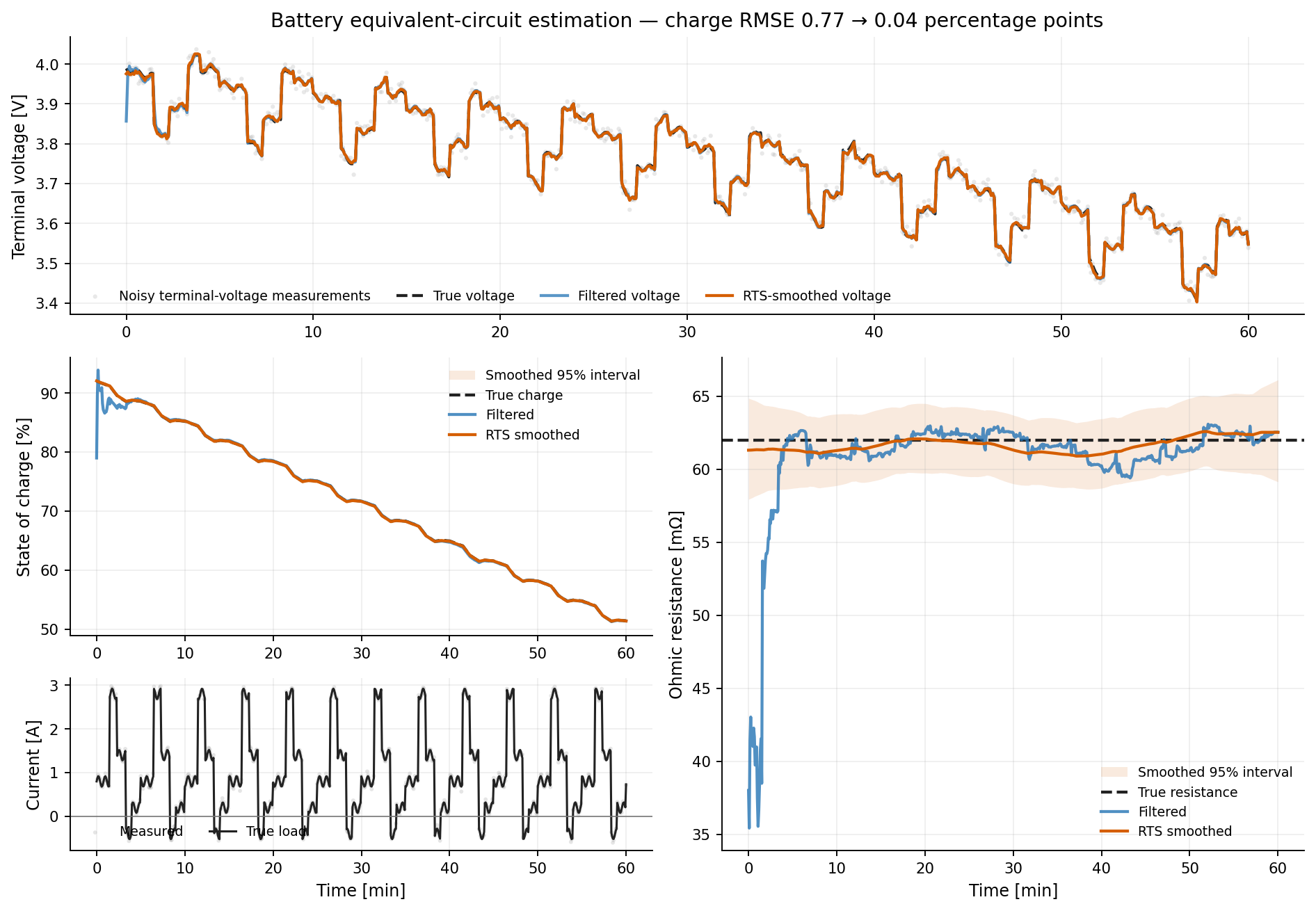
Battery state-of-charge and resistance estimation
This example uses a first-order Thevenin equivalent circuit to infer a lithium-ion cell's state of charge and ohmic internal resistance. The state is
x = [q, vₚ, log(R₀), I],
where q is fractional charge, vₚ is the voltage across a polarization RC
branch, and I is positive during discharge. Resistance is represented in log
space so its estimate remains positive. For cell capacity Q, polarization
resistance R₁, and time constant τ, the discrete transition is
q'  = q - dt I / (3600 Q)
vₚ' = exp(-dt/τ) vₚ + R₁ (1 - exp(-dt/τ)) I.
The available sensors measure noisy terminal voltage and noisy load current:
V_terminal = OCV(q) - vₚ - R₀ I
z = [V_terminal, I] + noise.
The nonlinear open-circuit-voltage curve makes charge observable, while the
repeating discharge, pulse-load, rest, and regenerative portions of the drive
cycle excite the instantaneous voltage drop needed to identify R₀. The
filter starts with deliberately biased charge and resistance estimates. RTS
smoothing then uses the entire one-hour experiment to reconstruct the early
charge state and resistance. The default uses unscented propagation, and
analytic Jacobians are included and tested for extended filtering and
smoothing as well.
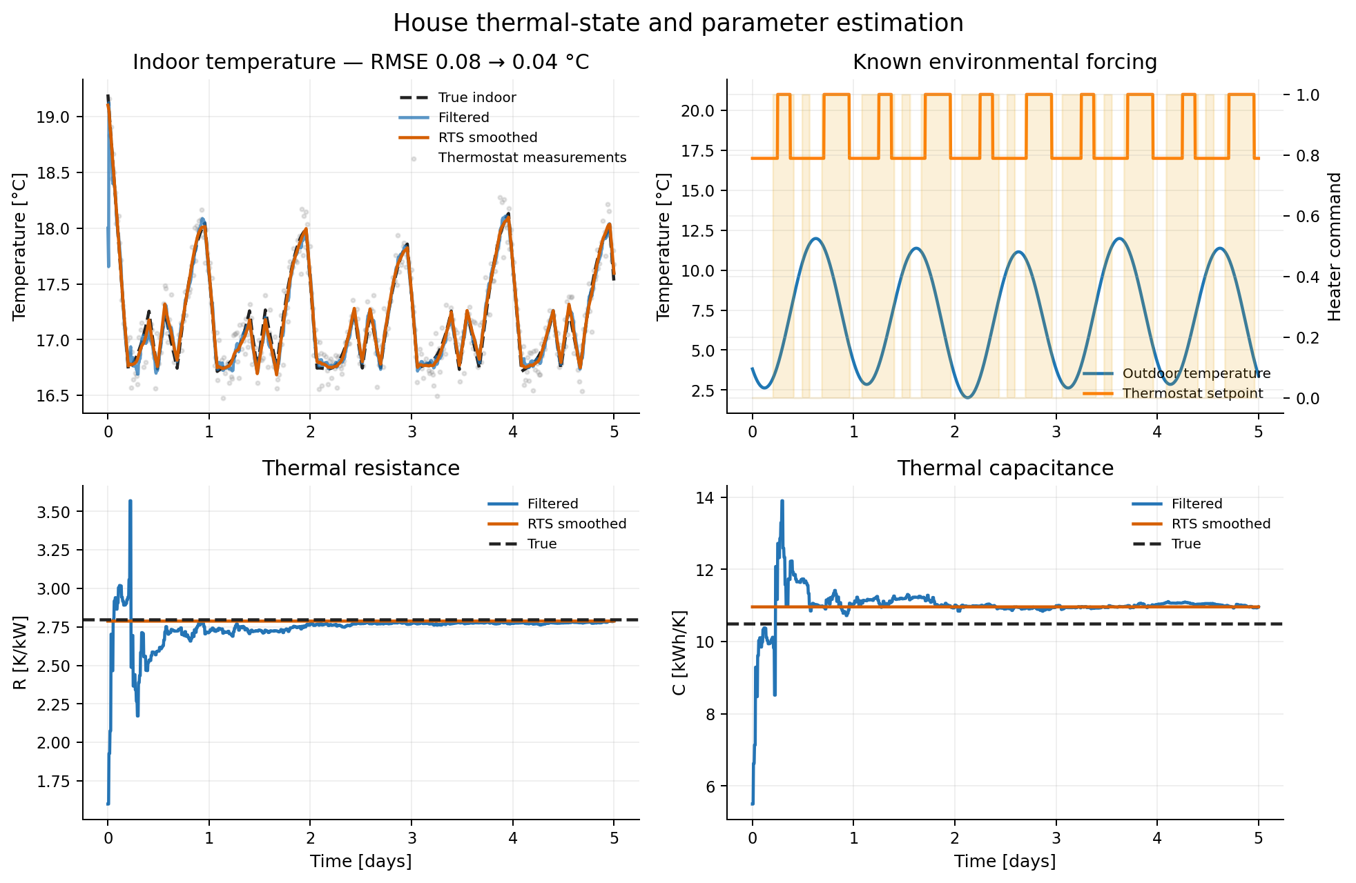
House thermal-parameter inference
A one-zone RC building model infers indoor temperature, insulation resistance, and thermal capacitance from thermostat measurements, known outdoor weather, and heater commands over five simulated days.
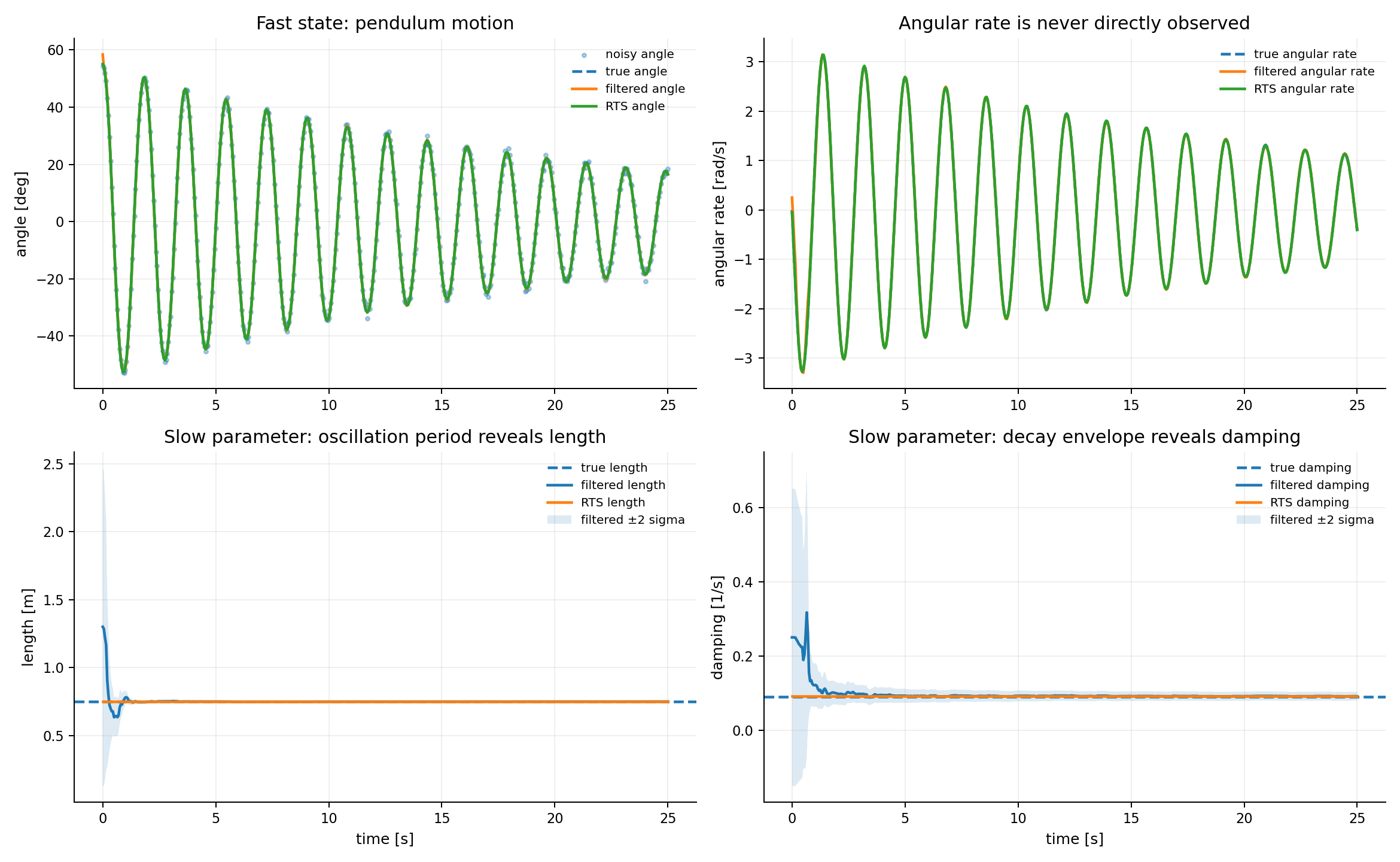
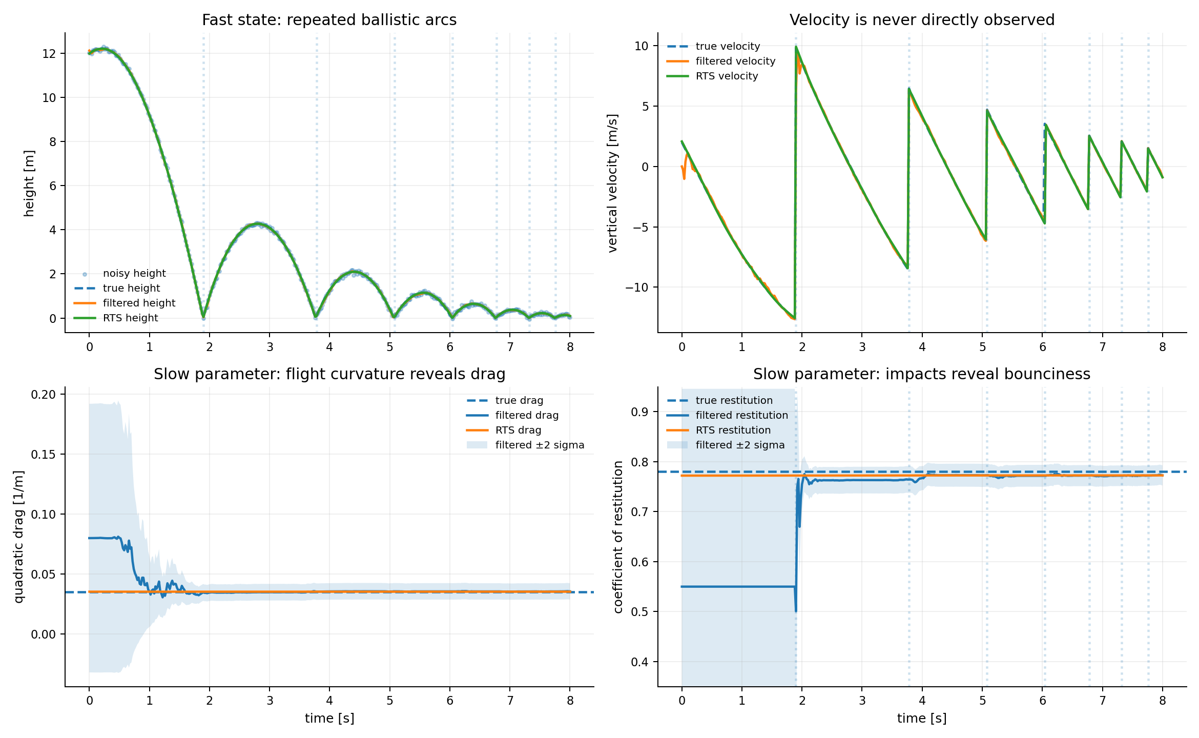
Pendulum and bouncing-ball parameter inference
The pendulum jointly estimates motion, length, and damping from noisy angle. The hybrid bouncing-ball example learns quadratic drag during flight and the coefficient of restitution at impacts from height measurements alone.
| Pendulum length and damping | Ball drag and restitution |
|---|---|
 |
 |
Sloshing fill-level inference
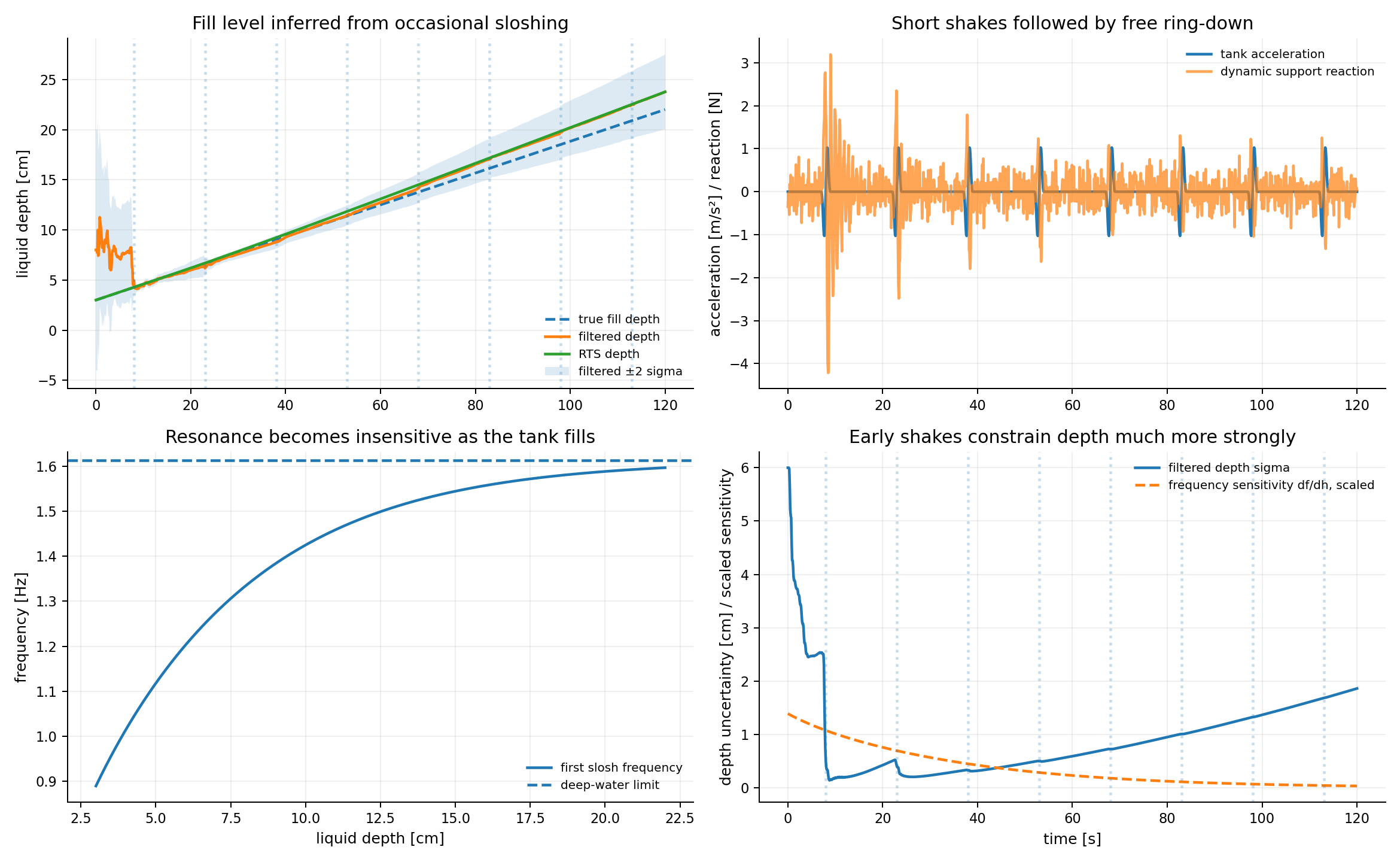
Short tank-acceleration pulses excite a depth-dependent liquid resonance. The filter infers fill depth and filling rate from dynamic support-load response without observing level, liquid mass, or static tank weight.
Active-suspension road-profile inference
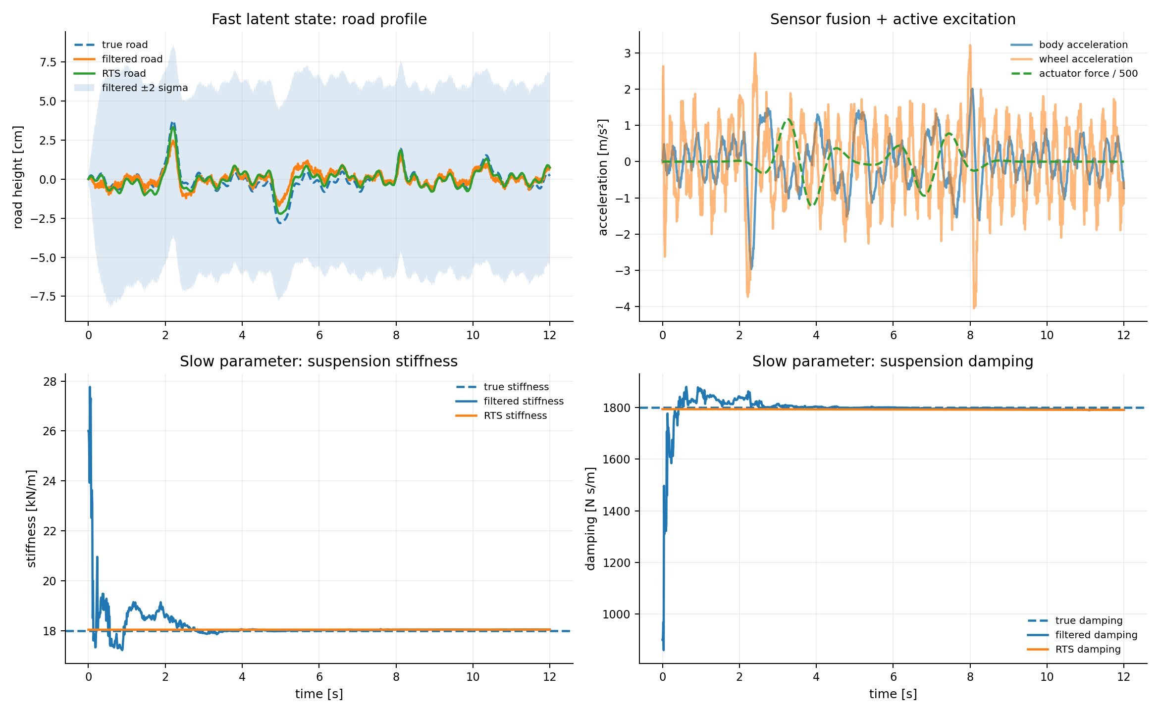
A quarter-car model combines sprung/unsprung accelerations, suspension travel, and measured actuator force to reconstruct road height while learning suspension stiffness and damping on separate fast and slow timescales.
Vehicle coast-down parameter inference
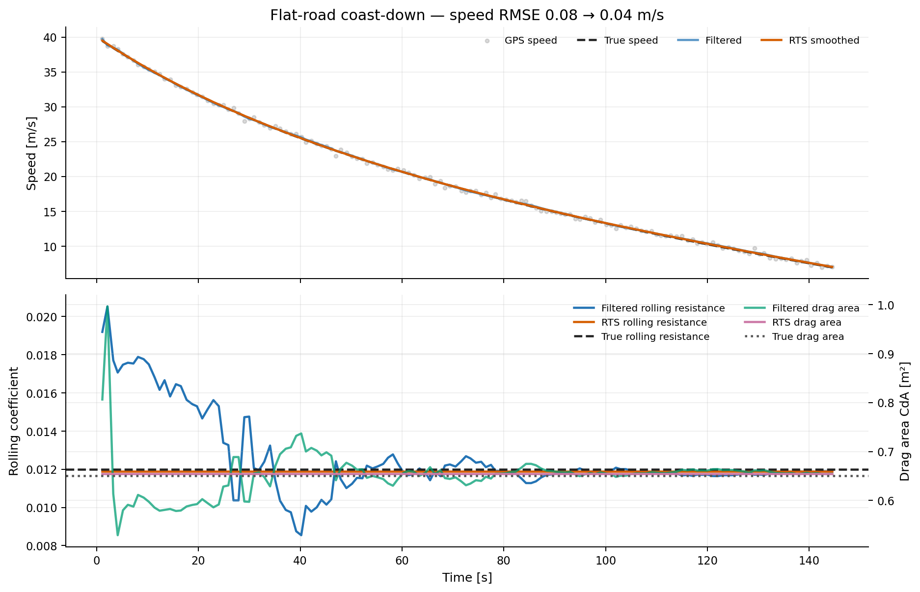
A flat-road coast-down separates nearly constant rolling resistance from speed-squared aerodynamic drag using only noisy GPS speed over a broad speed range.
Wheel-slip estimation
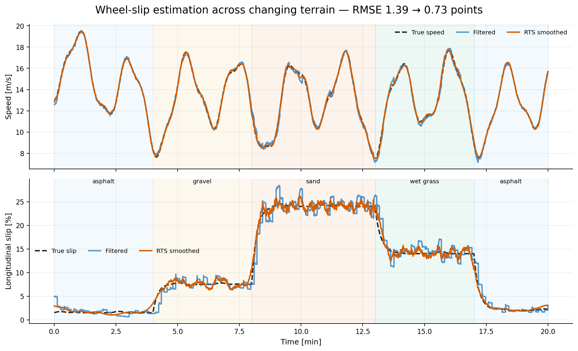
This example estimates changing longitudinal slip while traversing asphalt, gravel, sand, and wet grass without giving terrain labels to the filter.
Measurement-model lessons
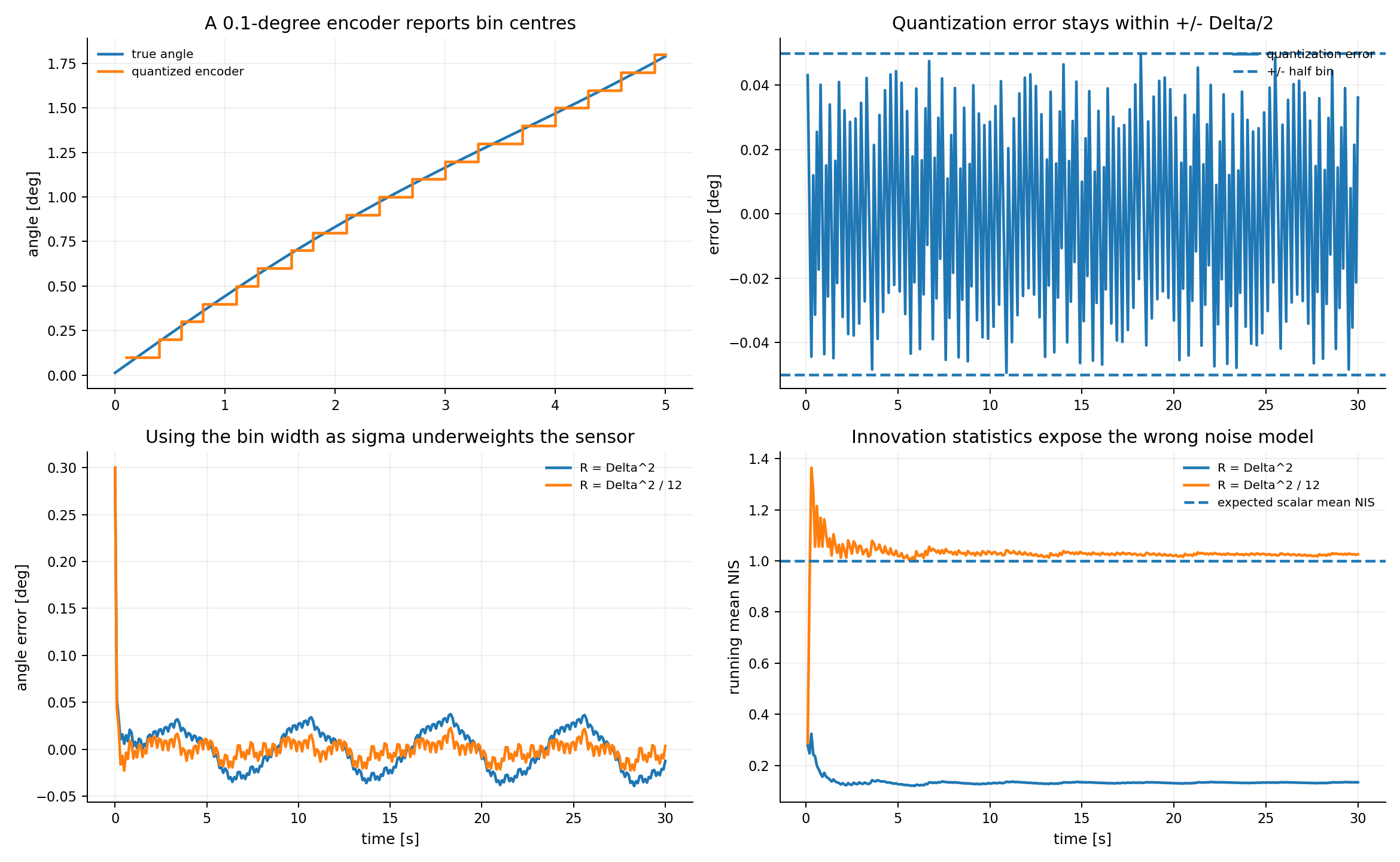
Quantization-noise covariance
Two otherwise identical filters compare R = Delta^2 against the uniform-bin
model R = Delta^2 / 12 for a quantized encoder. Tracking error and normalized
innovation squared show why sensor resolution is not one standard deviation.
Binary-packet channel tracking
A one-state filter reconstructs continuous link margin from packet success and failure bits alone. The example documents its assumed-Gaussian approximation to a Bernoulli likelihood and shows why bits are most informative near the decoder threshold.
Tests
The suite contains analytic linear-Gaussian regression tests and integration tests covering filtering, smoothing, irregular observation timing, batched observations, and both propagation modes.
python -m pip install -e '.[test]'
python -m pytest
Pytest measures branch coverage for the bayesfilter package and enforces the
minimum configured in pytest.ini.
Package layout
bayesfilter/distributions.py: Gaussian distributions and sigma points.bayesfilter/model.py: State transition models.bayesfilter/observation.py: Observation models.bayesfilter/filtering.py: Bayesian prediction and update loops.bayesfilter/smoothing.py: RTS smoothing.bayesfilter/unscented.py: Unscented-transform utilities.examples/: Runnable tracking and rigid-body examples and their figures.tests/: Unit and integration tests.
License
BayesFilter is distributed under the MIT License. See LICENSE.
1 maintainer

Metadata
1 maintainer
Release files for bayesfilter 0.2.0
For a detailed explanation of source distributions (sdists) and built distributions (wheels), please see the package formats documentation.
Source distribution (sdist)
| File | Size | Uploaded | |
|---|---|---|---|
| bayesfilter-0.2.0.tar.gz | 11.6 MB | Details |
Built distribution (wheel)
| File | Interpreter | ABI | Platform | Reset |
|---|---|---|---|---|
| bayesfilter-0.2.0-py3-none-any.whl | Python 3 | none | any | Details |
Total release size: 11.6 MB
Release files / bayesfilter-0.2.0.tar.gz
| Download URL | bayesfilter-0.2.0.tar.gz |
|---|---|
| Size | 11.6 MB |
| Tags | Source |
|
SHA-256 checksum How to use checksums |
f852996421728aad38085a305e0a76bc34efdfe5c2faad1fd59882dbcab3020c
|
|
BLAKE2b-256 checksum How to use checksums |
2c9c1e40ae21d8d98c8ad686030e479a1836054d8f950ba6c62ae448481f6a8c
|
| Upload date | |
|
Uploaded using Trusted Publishing? What is trusted publishing? |
Yes |
| Uploaded via |
twine/7.0.0 CPython/3.13.14
|
Provenance
Provenance describes where a file came from. On PyPI, provenance is shared via attestations, which provide a verifiable record of the build or publishing details. View details, limitations and caveats.


PyPI Publish Attestation
PyPI verified that this artifact, at this checksum, originated from the publisher listed below.
Signed by GitHub Actions, verified by PyPI on Sep 28, 2026.
Transparency logRelease files / bayesfilter-0.2.0-py3-none-any.whl
| Download URL | bayesfilter-0.2.0-py3-none-any.whl |
|---|---|
| Size | 23.1 kB |
| Tags | Python 3 |
|
SHA-256 checksum How to use checksums |
553394816af89cb87994a13ab6b591df727763073e13bd92db9775e8252eb1a7
|
|
BLAKE2b-256 checksum How to use checksums |
63dc9bdb4662a1590adf9c3b67fb998a07a01867235ac2a06e131a484124db41
|
| Upload date | |
|
Uploaded using Trusted Publishing? What is trusted publishing? |
Yes |
| Uploaded via |
twine/7.0.0 CPython/3.13.14
|
Provenance
Provenance describes where a file came from. On PyPI, provenance is shared via attestations, which provide a verifiable record of the build or publishing details. View details, limitations and caveats.
PyPI Publish Attestation
PyPI verified that this artifact, at this checksum, originated from the publisher listed below.
Signed by GitHub Actions, verified by PyPI on Sep 28, 2026.
Transparency log













