Performant numerical solutions of the paraxial ray equation

Project description
BeLinear
Performant numerical solutions of the paraxial ray equation.

Installation and Testing
Please install the package using pip.
pip install <unzipped belinear directory>
Once setup the package can be tested using python's unittest framework.
(mainenv) [cmpierce@turing ~]$ python -m unittest belinear.tests
........
----------------------------------------------------------------------
Ran 8 tests in 0.136s

OK
You should see an indication that all tests pass successfully.
Quick-start Guide
To calculate linear transfer matrices, you're going to need fieldmaps for all of the elements in your system. We're going to pick up the script after you have already calculated the fields (Ez and Bz) along the axis of the beamline. The fields and positions must be in SI units: MV/m, Tesla, and meters. I'll be using the following fields as an examples.
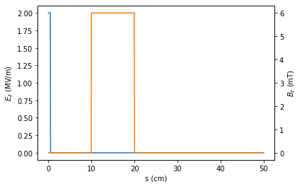
Once we have the fields, we can make the call to the solver and get the transfer matrix. The transfer matrix will be returned in [x, px] phase space as opposed to [x, x'] trace space which is common in accelerator physics. This is done because the angle x' becomes ill-determined when particles have zero longitudinal momentum as is the case at the start of integration in guns.
The solver accepts a step size h in meters which will determine the accuracy of the resulting matrices. See the section on convergence properties for a detailed discussion of how to choose this. In my experience, setting h = ~1e-6 is suitable for most accelerator physics applications.
The following example will setup some test fields and then solve for the resulting transfer matrix.
# Load belinear and numpy
import belinear
import numpy as np

# Compute the fields on axis (replace with your code)
z   = np.linspace(0, 0.5, 1000)
Ez = (z_raw<0.005)*10e3/5e-3
Bz = np.bitwise_and(z_raw > 0.1, z_raw < 0.2) * 6e-3

# Set the solver step size
h = 5e-6

# Solver for the transfer matrix
M = belinear.get_M(z, Ez, Bz, h)
Note: this will start the particles with no longitudinal velocity and so we require that Ez(z=0) != 0. To start with non-zero longitudinal energy, set the appropriate option.
# Calculate the transport matrix
M = belinear.get_M(z, Ez, Bz, h, gamma_initial=2)
BeLinear also supports multiple ODE solvers. We have been using the default option which is the midpoint method. This is expected to be the best option for most cases, however you may change which solver is used with the optional argument method.
# Calculate the linear transport matrix
M = belinear.get_M(z, Ez, Bz, h, method='<method name>')
The solvers supported by BeLinear are:
- "midpoint" - The midpoint rule or modified Euler's method is a symplectic integrator with second order global convergence. It shows excellent accuracy for Hamiltonian systems with a low number of steps and preserves the symplectic form. This is the default option in BeLinear and shows the best convergence for regularly used field configurations.
- "implicit_euler" - This method is the well known implicit Euler's method. It's has first order global convergence and better stability than forwards Euler for some systems.
- "constant_field" - Adapted from the paper "Gulliford, C., & Bazarov, I. (2012). PRAB, 15(2), 024002". It iterates the solution to [x1'(z), x2'(z)] = [[A, B], [C, D]]*[x1(z), x2(z)] for values of A, B, C, and D computed from the fields. That is, it assumes constant coefficients in the ODE, but not necessarily constant fields since the coefficients also depend on gamma which changes in the presence of constant E fields.
BeLinear also support cumulative output of the transfer matrices as one big numpy array of shape (2,2,N). This function has all the same options as the normal solver call. The following example will generate the cumulative matrices and plot all of them.
# Load belinear and numpy
import belinear
import numpy as np
import matplotlib.pyplot as plt

# Compute the fields on axis (replace with your code)
z   = np.linspace(0, 0.5, 1000)
Ez = (z_raw<0.005)*10e3/5e-3
Bz = np.bitwise_and(z_raw > 0.1, z_raw < 0.2) * 6e-3

# Set the solver step size
h = 5e-6

# Solver for the transfer matrices
M = belinear.get_cum_M(z, Ez, Bz, 5e-6)

# Get the positions matrices are output at
zM = np.arange(min(z), max(z), h)

# Plot the resulting dynamics
plt.plot(zM*1e2, M[0,0,:], c="C0")
plt.xlabel("s (cm)")
plt.ylabel("$M_{11}$", c="C0")
plt.twinx()
plt.plot(zM*1e2, M[1,1,:], c="C1")
plt.ylabel("$M_{22}$", c="C1")
Plotting the matrix elements against position gives the following plot.
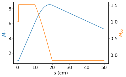
This is also useful for calculating beam size along the system as in the following example.
# Load belinear and numpy
import belinear
import numpy as np
import matplotlib.pyplot as plt
# Compute the fields on axis (replace with your code)
z = np.linspace(0, 0.5, 1000)
Ez = (z_raw<0.005)*10e3/5e-3
Bz = np.bitwise_and(z_raw > 0.1, z_raw < 0.2) * 6e-3
# Set the solver step size
h = 5e-6
# Solver for the transfer matrices
M = belinear.get_cum_M(z, Ez, Bz, 5e-6)
# Get the positions matrices are output at
zM = np.arange(min(z), max(z), h)
# Set initial beam parameters (25 um RMS spot size, 25 meV MTE)
# and solve for them along beamline
x = np.array([25e-6, np.sqrt(25e-3/511e3)])
xM = np.sqrt((x**2 @ (M**2).T).T)
# Plot beam size
plt.plot(zM*1e2, xM[0,:]*1e6)
plt.xlabel("s (cm)")
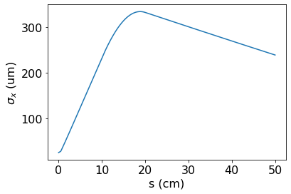
plt.ylabel("$\sigma_x$ (um)")
This should output the following plot of beam size.
Convergence Properties
To test the convergence properties run the solver with a smaller step size than you would reasonably use (h = 1e-8 m for instance) and use the output as a "ground truth" results of what the matrix should be. Run the solver again for you system while changing the step size and monitor the error. If your step size was small enough in the previous step then you see asymptotically power law convergence of the global error. As an example, I have computed the maximum global error vs step size for the field map at the top of the file and for the three solvers included in BeLinear.
# Load belinear and numpy
import belinear
import numpy as np

# Compute the fields on axis (replace with your code)
z   = np.linspace(0, 0.5, 1000)
Ez = (z_raw<0.005)*10e3/5e-3
Bz = np.bitwise_and(z_raw > 0.1, z_raw < 0.2) * 6e-3

# Set the solver step size for our reference matrix
h_ref = 1e-8

# Solver for the transfer matrices
M_ref = belinear.get_M(z, Ez, Bz, h_ref)

# Get matrices for a wide variety of step size
hs = np.exp(np.linspace(np.log(1e-7), np.log(1e-4), 25))
M_midpoint = np.array([belinear.get_M(z, Ez, Bz, h, method="midpoint") for h in hs])
M_implicit_euler = np.array([belinear.get_M(z, Ez, Bz, h, method="implicit_euler") for h in hs])
M_constant_field = np.array([belinear.get_M(z, Ez, Bz, h, method="constant_field") for h in hs])

# Compute the max relative error
err_midpoint = np.abs((M_midpoint-M_ref)/M_ref).max(axis=1).max(axis=1)
err_implicit_euler = np.abs((M_implicit_euler-M_ref)/M_ref).max(axis=1).max(axis=1)
err_constant_field = np.abs((M_constant_field-M_ref)/M_ref).max(axis=1).max(axis=1)

# Plot the relative error
plt.loglog(hs, err_midpoint, ls="none", marker="x", label="Midpoint")
plt.loglog(hs, err_implicit_euler, ls="none", marker="x", label="Euler")
plt.loglog(hs, err_constant_field, ls="none", marker="x", label="Constant")
plt.xlabel("h (m)")
plt.ylabel("Max. Relative Error")
plt.legend()
This example will produce the following output.
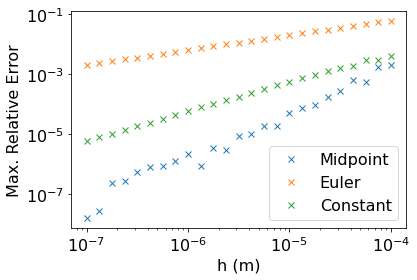
From this, the higher order convergence of the midpoint method is clear. The step size can now be selected based off of the trade-off between speed and accuracy. For many applications, a step size of between 1 um and 10 um will be adequate and provide excellent performance.
Reference
get_M(z, Ez, Bz, h, gamma_initial=1, method='midpoint')
Primary interface to the solver. Please call this from user code as opposed to the low level functions to calculate the linear transport matrices from the fields Ez and Bz sampled at points z. Convergence is controlled by the step size h.
Parameters
- z: array_like Positions of the field samples in meters.
- Ez: array_like The z component of the on-axis electric field in MV/m. An (n,) shape array.
- Bz: array_like The z component of the on-axis magnetic field in Tesla. An (n,) shape array.
- h: float Solver step size in meters.
- gamma_initial: float The relativistic gamma factor of the beam at the start of the region of integration
- method: str Which ODE solver to use. Options are "midpoint", "implicit_euler", or "constant_field"
Returns
- M: array_like The linear transport matrix in [x, px] phase space. A (2,2) numpy array.
get_cum_M(z, Ez, Bz, h, gamma_initial=1, method='midpoint')
The same solver function as "get_M" except that it will output the transfer matrices at every step taken by the solver. Useful for plotting particle trajectories.
Parameters
- z: array_like Positions of the field samples in meters.
- Ez: array_like The z component of the on-axis electric field in MV/m. An (n,) shape array.
- Bz: array_like The z component of the on-axis magnetic field in Tesla. An (n,) shape array.
- h: float Solver step size in meters.
- gamma_initial: float The relativistic gamma factor of the beam at the start of the region of integration
- method: str Which ODE solver to use. Options are "midpoint", "implicit_euler", or "constant_field"
Returns
- M_cum: array_like The transfer matrices in phase space ([x, px]) output at every step from the solver. A (2,2,n) numpy array.
Release history Release notifications | RSS feed


Download files
Download the file for your platform. If you're not sure which to choose, learn more about installing packages.
Source Distribution
Built Distribution
Filter files by name, interpreter, ABI, and platform.
If you're not sure about the file name format, learn more about wheel file names.
Copy a direct link to the current filters
File details
Details for the file belinear-1.1.tar.gz.
File metadata
- Download URL: belinear-1.1.tar.gz
- Upload date:
- Size: 8.4 kB
- Tags: Source
- Uploaded using Trusted Publishing? No
- Uploaded via: twine/1.15.0 pkginfo/1.5.0.1 requests/2.23.0 setuptools/40.6.3 requests-toolbelt/0.9.1 tqdm/4.46.0 CPython/3.5.6
File hashes
| Algorithm | Hash digest | |
|---|---|---|
| SHA256 |
58c6d0b9c114f8d0f8427df2a2cbeb1e08e3c633cb5608a56b7488f5d2ec4aca
|
|
| MD5 |
23f6cf395a9c0a3482766d8cb2ae48e3
|
|
| BLAKE2b-256 |
ed88fd74da430b0ecf63cfc810d54b192756a72eea1c1cea2b730975ccab2d75
|
File details
Details for the file belinear-1.1-py3-none-any.whl.
File metadata
- Download URL: belinear-1.1-py3-none-any.whl
- Upload date:
- Size: 2.9 MB
- Tags: Python 3
- Uploaded using Trusted Publishing? No
- Uploaded via: twine/1.15.0 pkginfo/1.5.0.1 requests/2.23.0 setuptools/40.6.3 requests-toolbelt/0.9.1 tqdm/4.46.0 CPython/3.5.6
File hashes
| Algorithm | Hash digest | |
|---|---|---|
| SHA256 |
f12f54660eb8a4f5537c8de8b838ef5d1644aaf36f848a470dd869cf5b04c25d
|
|
| MD5 |
032ed5700b2948445cf624471f515a0f
|
|
| BLAKE2b-256 |
61f539fa13a414a01f418ff878584714ae041ff496d3e70cbc89065cf17238d2
|


