BetaEarth: AlphaEarth Embedding Emulator

Project description


Embedding Sentinel-2 and Sentinel-1 with a Little Help of AlphaEarth
What is BetaEarth?
Open-Source Embedding Product Emulator
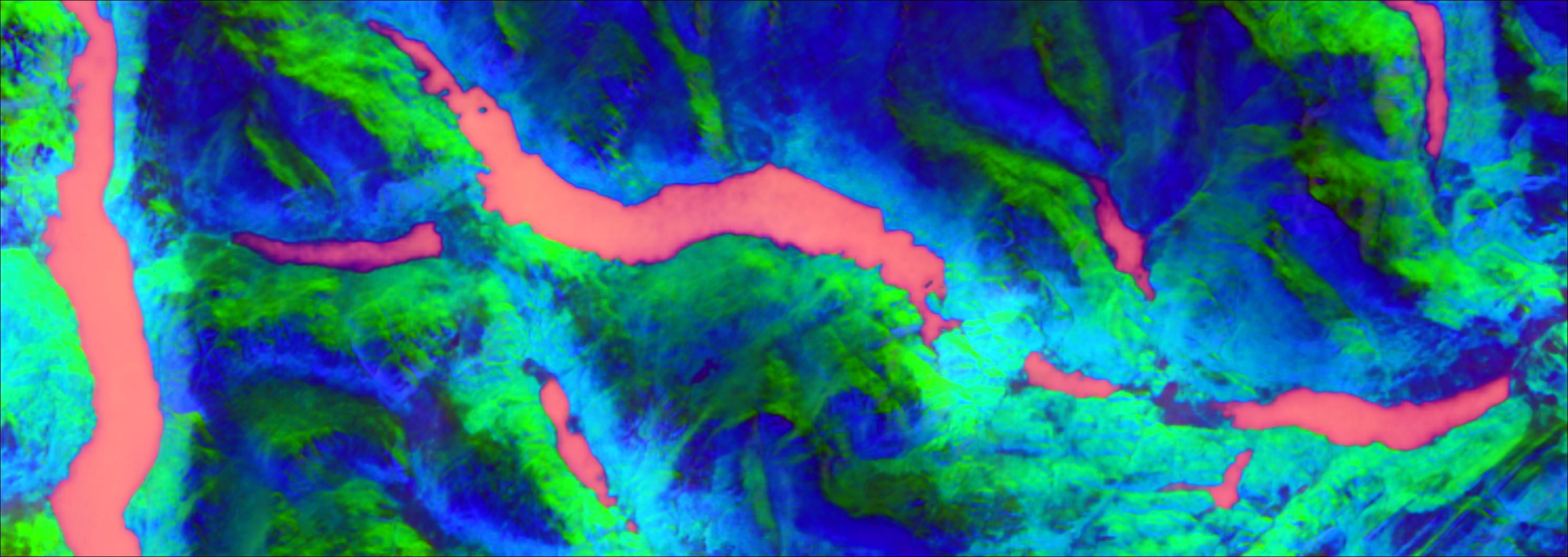
BetaEarth is an open-source model that produces dense 10m geospatial embedding fields from Sentinel-2 and Sentinel-1 imagery. It is trained to reproduce the outputs of AlphaEarth Foundations (AEF) — a closed-source embedding model released by Google and Google DeepMind — using only AEF's publicly available precomputed embeddings as supervision.
BetaEarth has no access to AEF's weights or architecture. It is an independent model, not a variant or extension of AEF. Its performance can often be inferior to AlphaEarth but it can be computed at a lower cost and with transparent access to the full data workflow, including the model.
Why does this matter?
- Reproducibility: AEF embeddings cannot be generated for new data without Google Earth Engine access. BetaEarth can run locally on any Sentinel-2/S1 imagery.
- Auditability: BetaEarth enables the community to probe a closed-source model's behaviour — identifying biases, modality sensitivities, and failure modes — without direct model access.
- Security research: This work demonstrates that releasing embeddings may not be a risk-free alternative to releasing model weights.
Generate embeddings for any area
Four entry points, from zero-install to fully scripted.
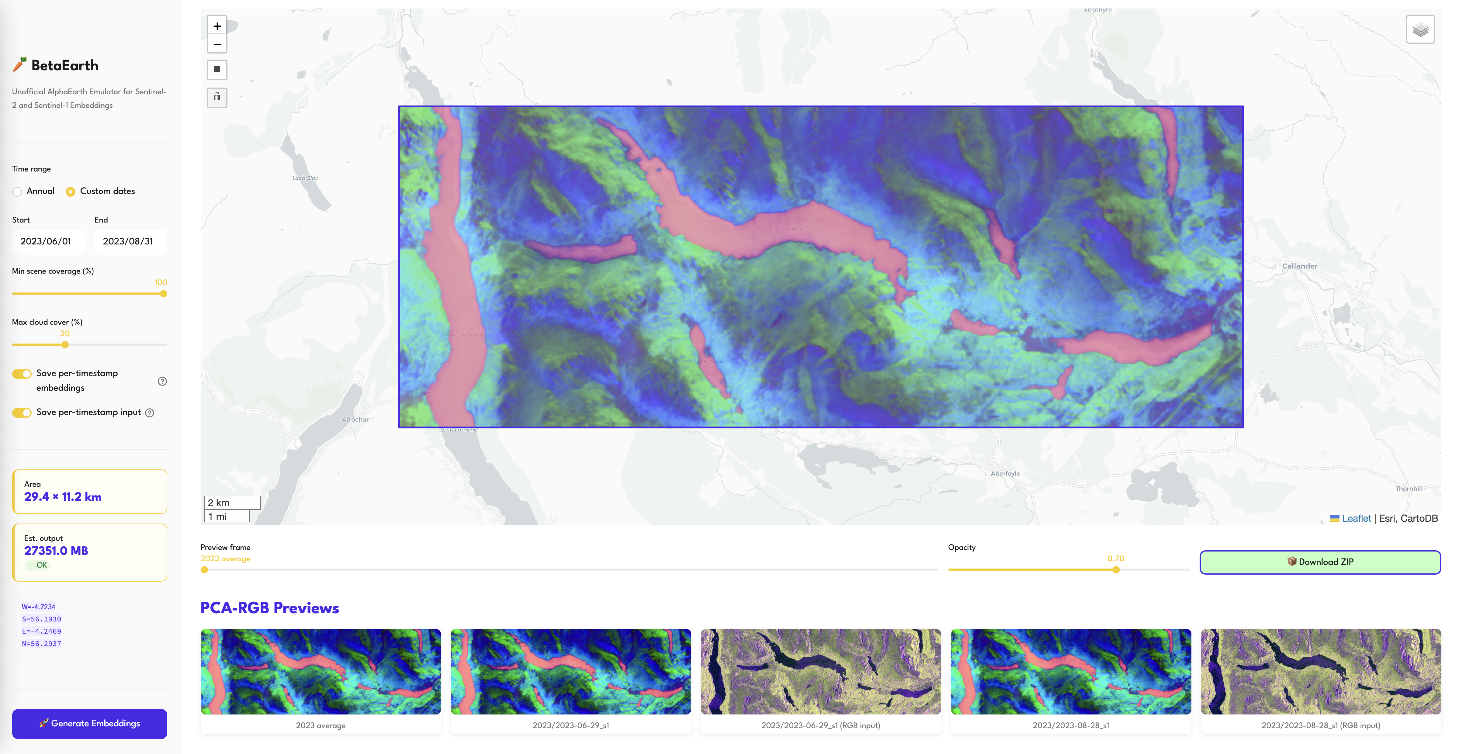
1. Hosted demo (no install)
Pick a bounding box on a map, click run: huggingface.co/spaces/asterisk-labs/betaearth. Free tier is CPU-only and caps total output at 3 GB.
2. Colab notebook (recommended for first try)
examples/generate_demo.ipynb walks through the full pipeline in a notebook: pip install betaearth[generate], pick an AOI on an interactive map, run one cell, visualise annual + per-timestamp PCA-RGB previews side-by-side. Uses Colab's free T4 GPU.
3. Command-line generation (the main path for real work)
betaearth-generate ships with the package and drives the same pipeline: download Sentinel-2 L2A + Sentinel-1 RTC + COP-DEM from Planetary Computer, run tiled inference, write an annual 64-band COG plus a full provenance manifest per year.
pip install 'betaearth[generate]'

# By bounding box (W S E N), one or more years
betaearth-generate --bbox 13.1 48.7 13.8 49.2 --years 2020 2021 2022 2023 2024 2025 \
    --output_dir outputs/bavarian_forest

# By OSM relation id (resolved to its bbox)
betaearth-generate --osm_relation 1864214 --years 2024 --output_dir outputs/bav
No API keys needed — Planetary Computer is publicly accessible. A CUDA GPU is used automatically if available; CPU works but is slower. Each run produces, per year:
| File | Description |
|---|---|
{year}.tif |
64-band annual average embedding (L2-normalised per pixel), COG |
{year}_preview_pca.png |
3-band PCA-RGB quick-look of the annual mosaic |
{year}_manifest.json |
Provenance: model repo + version, CRS/bounds/shape, acquisition params, full STAC id list of every scene used (cloud cover, coverage, S1 orbit/polarisation, ...) |
{year}_files/{date}_{sensor}/ |
Optional per-scene outputs, only with --save_per_timestamp_embedding / --save_scenes |
The manifest is deliberately verbose so any downstream user of the embedding can verify exactly which Sentinel products fed into it. Import betaearth.generate for the Python API that backs the CLI; a minimal scripted example is in examples/predict.py.
4. Streamlit app (local)
The same app as the hosted Space, run on your own compute:
git clone https://github.com/asterisk-labs/beta-earth
cd beta-earth
pip install 'betaearth[demo]'
streamlit run demo/app.py
Then open http://localhost:8501 in your browser. Raise the 3 GB cap via env var:
BETAEARTH_MAX_OUTPUT_MB=50000 streamlit run demo/app.py # 50 GB ceiling
Models
We release 8 model variants spanning different trade-offs between quality, parameter efficiency, and input requirements.
Main results (6,200-tile test set)
| Model | Test Cos Sim | Std | LULC Acc | Model Size | Inputs |
|---|---|---|---|---|---|
| SF curriculum (robust) | 0.873 | 0.109 | 0.833 | 104.8M | Any subset of S2/S1/DEM + DOY |
| SF frozen+FiLM (reinit) | 0.886 | 0.098 | 0.873 | 104.8M | S2 L1C+L2A, S1, DEM, DOY |
| SF frozen+FiLM (hilr) | 0.886 | 0.099 | 0.866 | 104.8M | S2 L1C+L2A, S1, DEM, DOY |
| SF from scratch+FiLM | 0.883 | --- | 0.835 | 104.8M | S2 L1C+L2A, S1, DEM, DOY |
| SF no FiLM (ISPRS) | 0.880 | 0.101 | 0.869 | 104.8M | S2 L1C+L2A, S1, DEM |
| DINOv3 ViT-L/16 (sat) | 0.874 | 0.100 | 0.870 | 304M | 6 primitives + DOY |
| DINOv3 ViT-S/16 (nat) | 0.861 | 0.109 | 0.863 | 23.8M | 6 primitives + DOY |
| SF RGB-only+FiLM | 0.836 | --- | 0.823 | 26.3M | S2 RGB, DOY |
| Real AlphaEarth (ceiling) | --- | --- | 0.889 | --- | --- |
The curriculum (robust) model handles any modality subset gracefully:
| Input subset | Cosine sim |
|---|---|
| All modalities | 0.873 |
| L1C only | 0.806 |
| L2A only | 0.755 |
| S1 only | 0.712 |
| DEM only | 0.609 |
Which model should I use?
| Use case | Recommended model | Why |
|---|---|---|
| General use (default) | SF curriculum (robust) | Works with any input subset; best for real-world deployment |
| Maximum quality | SF frozen+FiLM (reinit) | Highest cos sim (0.886) — requires all 4 modalities |
| No timestamp needed | SF no FiLM (ISPRS) | Does not require day-of-year input; still achieves 0.880 |
| Lightweight / edge | DINOv3 ViT-S/16 | 23.8M params, good quality (0.861) |
| Minimal data requirements | SF RGB-only+FiLM | Only needs 3-band RGB + day-of-year |
| Research / ablation | SF frozen+FiLM (hilr) | Alternative fusion strategy for comparison |
Architecture overview
DINOv3 models use a single shared frozen DINOv3 backbone applied to 3-band spectral primitives:
| Primitive | Bands | Captures |
|---|---|---|
| True-colour RGB | B04/B03/B02 | Visual texture, built environment |
| False-colour IR | B08/B04/B03 | Vegetation health (NIR) |
| SWIR composite | B12/B11/B04 | Moisture, bare soil, burn scars |
| Red-edge | B07/B06/B05 | Canopy structure, chlorophyll |
| SAR | VV/VH/ratio | Structure, moisture (from S1) |
| Topography | Elevation/Slope/Aspect | Terrain (from COP-DEM) |
Primitives are fused via permutation-invariant cross-attention (SetFusion).
SegFormer models use 4 separate MiT-B2 encoders processing each modality's raw bands natively (9ch S2-L1C, 9ch S2-L2A, 2ch S1, 1ch DEM), with channel concatenation fusion.
All models use FiLM temporal conditioning (day-of-year modulation) except the ISPRS baseline.
Key findings
- Temporal conditioning as spectral compensation: FiLM importance scales inversely with spectral access — RGB-only (22pp) > DINOv3 (18pp) > SegFormer scratch (14pp) > frozen SegFormer (5pp).
- Multi-temporal averaging of 4+ observations improves emulation by up to +13pp over single timestamps, with the benefit biome-dependent (gap-fill wins in boreal regions; S2-only wins in arid/temperate).
- Predicted embeddings retain 97% of downstream LULC classification accuracy and are robust to 32x compression.
Model Properties
| Property | Value |
|---|---|
| Output | Dense embedding field — (H, W, 64) per tile at 10m resolution |
| Output normalisation | L2-normalised per pixel (unit vectors on S^63) |
| Quantisation | Original AEF: int8 on S^63; BetaEarth outputs float32 |
| Tile size | 10.68 x 10.68 km (1068 x 1068 px), Major TOM grid |
| Training data | 62,489 Major TOM grid cells (49,991 train / 6,248 val / 6,250 test) |
| Loss | Cosine similarity + 0.1 * MSE, masked to valid pixels |
Quickstart
pip install betaearth
from betaearth import BetaEarth

model = BetaEarth.from_pretrained()  # default: robust variant
# BetaEarth(params=104.8M, device=cuda)

# All inputs are raw (unnormalised) — preprocessing is handled internally
embedding = model.predict(
    s2_l2a=s2_l2a,   # (9, H, W) uint16 DN (~0-10000)
    s2_l1c=s2_l1c,   # (9, H, W) uint16 DN (~0-10000)
    s1=s1,            # (2, H, W) float32 linear power
    dem=dem,          # (1, H, W) float32 elevation in meters
    doy=182,          # day of year (1-366)
)
# embedding: (H, W, 64) float32 numpy array, L2-normalised per pixel
Any modality can be omitted — the model handles missing inputs via zeroed features:
# S2-only (no S1, no DEM)
emb = model.predict(s2_l2a=s2_l2a, doy=182)

# S2 + DEM, no S1
emb = model.predict(s2_l2a=s2_l2a, dem=dem, doy=182)
Multi-temporal averaging
import numpy as np

preds = []
for s2, s1, doy in zip(s2_timeseries, s1_timeseries, doys):
    pred = model.predict(s2_l2a=s2, s1=s1, dem=dem, doy=doy)
    preds.append(pred)

# Simple averaging — saturates at ~4 observations
annual = np.mean(preds, axis=0)
annual /= np.linalg.norm(annual, axis=-1, keepdims=True)
Data Access
All training data is from the Major TOM community project and is freely available on HuggingFace:
| Dataset | Description |
|---|---|
| Major-TOM/Core-S2-L2A | Sentinel-2 L2A imagery |
| Major-TOM/Core-S2-L1C | Sentinel-2 L1C imagery |
| Major-TOM/Core-S1-RTC | Sentinel-1 RTC imagery |
| Major-TOM/Core-AlphaEarth-Embeddings | AEF target embeddings |
Data normalisation
All input data should be stored as raw values. Normalisation happens inside the model:
- S2 L1C/L2A: uint16 DN (0-10000+), divided by 10000 internally
- S1 RTC: linear power (float32, ~0-200), log-transformed internally
- COP-DEM: pre-normalised to [0, 1] before passing to the model
Important: S2 band order must follow Major TOM convention: [B02, B03, B04, B08, B05, B06, B07, B11, B12] (10m bands first, then 20m).
Reproduce
git clone https://github.com/asterisk-labs/beta-earth
cd beta-earth
conda env create -f environment.yml
conda activate betaearth

# Train (requires A100 GPU)
python train_multi.py --batch_size 8 --max_epochs 20

# SegFormer FiLM variants (frozen encoder)
python train_segformer_frozen_variants.py --ckpt checkpoints/isprs_v1_epoch19_0.875.ckpt

# Evaluate on test set
python run_evaluation.py --ckpt checkpoints/multi_final.ckpt

# Generate paper figures
python generate_figures.py
python plot_training_curves.py

# Multi-temporal experiments
python test_multitemporal.py --ckpt checkpoints/segformer_film_frozen_best.ckpt
See CHECKLIST.md for a full step-by-step guide to reproducing each experiment in the paper.
Citation
@inproceedings{czerkawski2026betaearth,
  title     = {BetaEarth: Emulating Closed-Source Earth Observation Models Through Their Public Embeddings},
  author    = {Czerkawski, Mikolaj},
  year      = {2026}
}
License and Attribution
BetaEarth model weights are released under CC-BY 4.0, matching the license of the AlphaEarth Foundations embedding archive used for training supervision.
Required attribution for AEF training data:
"The AlphaEarth Foundations Satellite Embedding dataset is produced by Google and Google DeepMind."
Training imagery is sourced from Major TOM (Apache 2.0) and Copernicus Sentinel (free and open access).


Download files
Download the file for your platform. If you're not sure which to choose, learn more about installing packages.
Source Distribution
Built Distribution
Filter files by name, interpreter, ABI, and platform.
If you're not sure about the file name format, learn more about wheel file names.
Copy a direct link to the current filters
File details
Details for the file betaearth-0.2.3.tar.gz.
File metadata
- Download URL: betaearth-0.2.3.tar.gz
- Upload date:
- Size: 30.3 kB
- Tags: Source
- Uploaded using Trusted Publishing? No
- Uploaded via: twine/6.1.0 CPython/3.8.17
File hashes
| Algorithm | Hash digest | |
|---|---|---|
| SHA256 |
ed4552844957ce5262aebb5435ad33a3263a4cf8cdbb74e0c5dbe71e84eab39d
|
|
| MD5 |
941e25192edcc52fb2b4b2e313261368
|
|
| BLAKE2b-256 |
1e7df164852d8554ca3a511ccc624df34f15fe139cf6d8e04c5890ccf5ed31a2
|
File details
Details for the file betaearth-0.2.3-py3-none-any.whl.
File metadata
- Download URL: betaearth-0.2.3-py3-none-any.whl
- Upload date:
- Size: 26.2 kB
- Tags: Python 3
- Uploaded using Trusted Publishing? No
- Uploaded via: twine/6.1.0 CPython/3.8.17
File hashes
| Algorithm | Hash digest | |
|---|---|---|
| SHA256 |
74e03166ae0d5f326ae5b8e83b71f4eb3941a33844e49b5ace09020bcded7579
|
|
| MD5 |
45d10529c5fe41b928efef797444c6c7
|
|
| BLAKE2b-256 |
6894a46937ff7b57830380be7ad2f6b708857bdde24fae804db54a97a39f09bc
|


