Bayesian layers for NumPyro and Jax
Verified details
These details have been verified by PyPIProject links
GitHub Statistics
Maintainers

Project description


BLayers
The missing layers package for Bayesian inference.
BLayers is in beta, errors are possible! We invite you to contribute on GitHub.
Write code immediately
pip install blayers
deps are: numpyro, jax, and optax.
Concept
Easily build Bayesian models from parts, abstract away the boilerplate, and tweak priors as you wish.
Inspiration from Keras and Tensorflow Probability, but made specifically for Numpyro + Jax.
BLayers provides tools to
- Quickly build Bayesian models from layers which encapsulate useful model parts
- Fit models either using Variational Inference (VI) or your sampling method of choice without having to rewrite models
- Write pure Numpyro to integrate with all of Numpyro's super powerful tools
- Add more complex layers (model parts) as you wish
- Fit models in a greater variety of ways with less code
The starting point
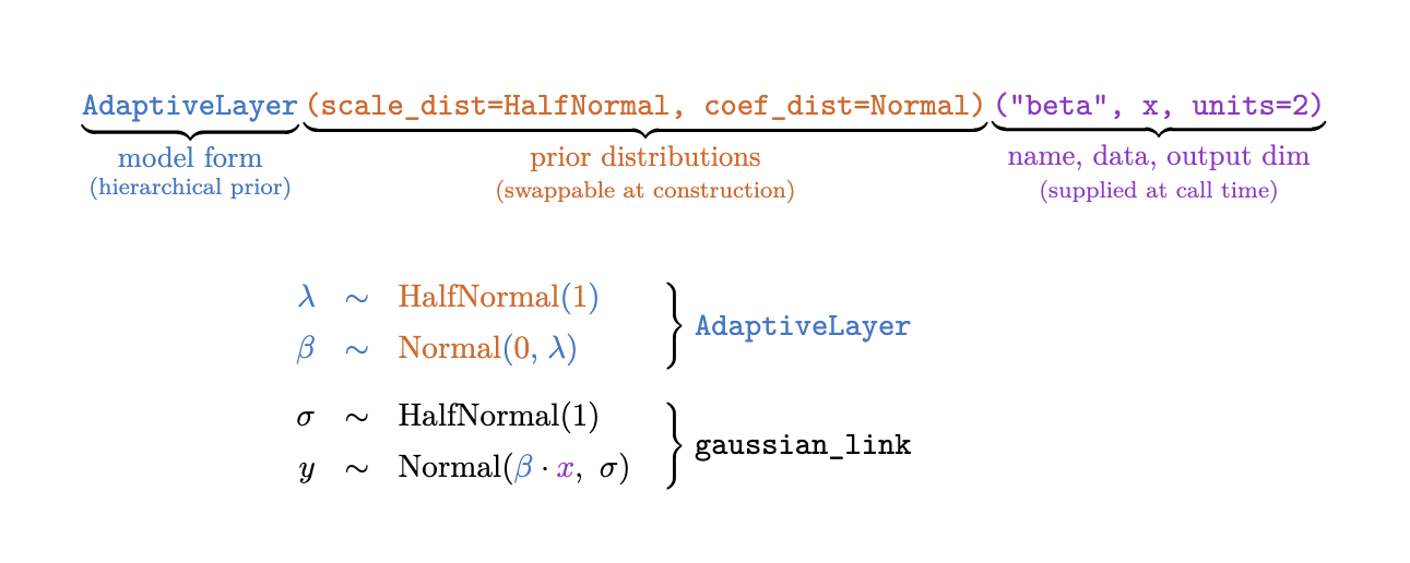
The simplest non-trivial (and most important!) Bayesian regression model form is the adaptive prior,
scale ~ HalfNormal(1)
beta  ~ Normal(0, scale)
y     ~ Normal(beta * x, 1)
BLayers encapsulates a generative model structure like this in a BLayer. The
fundamental building block is the AdaptiveLayer.
from blayers.layers import AdaptiveLayer
from blayers.links import gaussian_link

def model(x, y):
    mu = AdaptiveLayer()('mu', x)
    return gaussian_link(mu, y)
All AdaptiveLayer is doing is writing Numpyro for you under the hood. This
model is exactly equivalent to writing the following, just using way less code.
import jax.numpy as jnp
from numpyro import distributions, sample

def model(x, y):
    # Adaptive layer does all of this
    input_shape = x.shape[1]
    # adaptive prior
    scale = sample(
        name="scale",
        fn=distributions.HalfNormal(1.),
    )
    # beta coefficients for regression
    beta = sample(
        name="beta",
        fn=distributions.Normal(loc=0., scale=scale),
        sample_shape=(input_shape,),
    )
    mu = jnp.einsum('ij,j->i', x, beta)

    # the link function does this
    sigma = sample(name='sigma', fn=distributions.Exponential(1.))
    return sample('obs', distributions.Normal(mu, sigma), obs=y)
Mixing it up
The AdaptiveLayer is also fully parameterizable via arguments to the class, so let's say you wanted to change the model from
scale ~ HalfNormal(1)
beta  ~ Normal(0, scale)
y     ~ Normal(beta * x, 1)
to
scale ~ Exponential(1.)
beta  ~ LogNormal(0, scale)
y     ~ Normal(beta * x, 1)
you can just do this directly via arguments
from numpyro import distributions
from blayers.layers import AdaptiveLayer
from blayers.links import gaussian_link

def model(x, y):
    mu = AdaptiveLayer(
        scale_dist=distributions.Exponential,
        coef_dist=distributions.LogNormal,
        scale_kwargs={'rate': 1.},
        coef_kwargs={'loc': 0.}
    )('mu', x)
    return gaussian_link(mu, y)
"Factories"
Since Numpyro traces sample sites and doesn't record any parameters on the class, you can re-use with a particular generative model structure freely.
from numpyro import distributions
from blayers.layers import AdaptiveLayer
from blayers.links import gaussian_link

my_lognormal_layer = AdaptiveLayer(
    scale_dist=distributions.Exponential,
    coef_dist=distributions.LogNormal,
    scale_kwargs={'rate': 1.},
    coef_kwargs={'loc': 0.}
)

def model(x, y):
    mu = my_lognormal_layer('mu1', x) + my_lognormal_layer('mu2', x**2)
    return gaussian_link(mu, y)
Layers
The full set of layers included with BLayers:
AdaptiveLayer— Adaptive prior layer:scale ~ HalfNormal(1),beta ~ Normal(0, scale).FixedPriorLayer— Fixed prior over coefficients (e.g., Normal or Laplace), no hierarchical scale.InterceptLayer— Intercept-only layer (bias term).EmbeddingLayer— Bayesian embeddings for sparse categorical features.RandomEffectsLayer— Classical random-effects (embedding with output dim 1).FMLayer— Factorization Machine (order 2) for pairwise interaction terms.FM3Layer— Factorization Machine (order 3).LowRankInteractionLayer— Low-rank interaction between two feature sets.InteractionLayer— All pairwise interactions between two feature sets.BilinearLayer— Bilinear interaction:x^T W z.LowRankBilinearLayer— Low-rank bilinear interaction.RandomWalkLayer— Gaussian random walk prior over an ordered index (e.g., time).HorseshoeLayer— Horseshoe prior for sparse regression; global-local shrinkage via HalfCauchy.SpikeAndSlabLayer— Spike-and-slab prior;z ~ Beta(0.5, 0.5)inclusion weights times a configurable slab.AttentionLayer— Multi-head self-attention over the feature dimension with FT-Transformer tokenisation (Gorishniy et al. 2021).head_dimis per-head so total embedding dim ishead_dim * num_heads— adding heads increases capacity.
All layer prior kwargs are validated at construction time — bad kwargs raise TypeError immediately.
Links
We provide link helpers in links.py to reduce Numpyro boilerplate. Available links:
gaussian_link— Gaussian likelihood with configurable sigma prior (see below).lognormal_link— LogNormal likelihood with configurable sigma prior.logit_link— Bernoulli link for logistic regression.poisson_link— Poisson link with log-rate input.negative_binomial_link— NegativeBinomial2 for overdispersed counts; learned concentration viaExponential.ordinal_link— Cumulative logit / proportional odds for ordinal outcomes.zip_link— Zero-inflated Poisson for count data with excess zeros.beta_link— Beta regression for proportions strictly in (0, 1).
gaussian_link and lognormal_link
Both links are built on a common base and support three scale modes:
from blayers.layers import AdaptiveLayer
from blayers.links import gaussian_link

# Default: sigma ~ Exp(1) learned from data
gaussian_link(mu, y)

# Fixed known scale (e.g. from XGBoost quantile regression)
gaussian_link(mu, y, scale=pred_std)

# Learned scale from a layer — softplus applied internally for stable gradients
raw = AdaptiveLayer()("log_sigma", x)
gaussian_link(mu, y, untransformed_scale=raw)
Swap the sigma prior via functools.partial:
from functools import partial
import numpyro.distributions as dists
from blayers.layers import AdaptiveLayer
from blayers.links import gaussian_link

# HalfNormal prior instead of Exponential
hn_gaussian = partial(gaussian_link, sigma_dist=dists.HalfNormal, sigma_kwargs={"scale": 1.0})

def model(x, y=None):
    mu = AdaptiveLayer()("mu", x)
    return hn_gaussian(mu, y)
Splines
Non-linear transformations via B-splines. Compute the basis matrix once with make_knots + bspline_basis, then pass it to any layer.
from blayers.splines import make_knots, bspline_basis
from blayers.layers import AdaptiveLayer
from blayers.links import gaussian_link

knots = make_knots(x_train, num_knots=10)   # clamped knot vector from data quantiles

def model(x, y=None):
    B = bspline_basis(x, knots)             # (n, num_basis) design matrix
    f = AdaptiveLayer()("f", B)
    return gaussian_link(f, y)
Additive models are straightforward:
knots1 = make_knots(x1_train, num_knots=10)
knots2 = make_knots(x2_train, num_knots=10)

def model(x1, x2, y=None):
    f1 = AdaptiveLayer()("f1", bspline_basis(x1, knots1))
    f2 = AdaptiveLayer()("f2", bspline_basis(x2, knots2))
    return gaussian_link(f1 + f2, y)
fit() helpers
fit() handles the guide, ELBO, batching, and LR schedule. The same model runs unchanged under VI, MCMC, or SVGD.
from blayers.fit import fit
from blayers.decorators import autoreshape
from blayers.layers import AdaptiveLayer, InterceptLayer
from blayers.links import gaussian_link

@autoreshape
def model(x, y=None):
    mu = AdaptiveLayer()("beta", x)
    intercept = InterceptLayer()("intercept")
    return gaussian_link(mu + intercept, y)

# Variational Inference (default)
result = fit(model, y=y, num_steps=1000, batch_size=256, lr=0.01, x=X)

# MCMC
result = fit(model, y=y, method="mcmc", num_mcmc_samples=1000, num_warmup=500, x=X)

# SVGD
result = fit(model, y=y, method="svgd", num_steps=1000, num_particles=20, x=X)
result.predict() returns a Predictions object with .mean, .std, and .samples. result.summary() returns posterior stats per latent variable.
preds = result.predict(x=X, num_samples=500)
summary = result.summary(x=X)
Keyword arguments that are JAX arrays are treated as data (batched during training). Non-array kwargs are bound as constants.
Batched loss
The default Numpyro way to fit batched VI models is to use plate, which confuses
me a lot. Instead, BLayers provides Batched_Trace_ELBO which does not require
you to use plate to batch in VI. Just drop your model in.
from numpyro.infer import SVI
from numpyro.infer.autoguide import AutoDiagonalNormal
import optax
from blayers.vi_infer import Batched_Trace_ELBO, svi_run_batched

loss = Batched_Trace_ELBO(num_obs=len(y), batch_size=1000)
guide = AutoDiagonalNormal(model_fn)
svi = SVI(model_fn, guide, optax.adam(0.01), loss=loss)

svi_result = svi_run_batched(
    svi,
    rng_key,
    batch_size=1000,
    num_steps=500,
    **model_data,
)
⚠️⚠️⚠️ numpyro.plate + Batched_Trace_ELBO do not mix. ⚠️⚠️⚠️
Batched_Trace_ELBO is known to have issues when your model uses numpyro.plate. If your model needs plates, either:
- Batch via
plateand use the standardTrace_ELBO, or - Remove plates and use
Batched_Trace_ELBO+svi_run_batched.
Batched_Trace_ELBO will warn if your model has plates.
Reparameterizing
To fit MCMC models well it is crucial to reparameterize. BLayers helps you do this via @autoreparam, which automatically applies LocScaleReparam to all LocScale distributions in your model (Normal, LogNormal, StudentT, Cauchy, Laplace, Gumbel).
from numpyro.infer import MCMC, NUTS
from blayers.layers import AdaptiveLayer
from blayers.links import gaussian_link
from blayers.decorators import autoreparam

data = {...}

@autoreparam
def model(x, y):
    mu = AdaptiveLayer()('mu', x)
    return gaussian_link(mu, y)

kernel = NUTS(model)
mcmc = MCMC(
    kernel,
    num_warmup=500,
    num_samples=1000,
    num_chains=1,
    progress_bar=True,
)
mcmc.run(
    rng_key,
    **data,
)
Project details
Verified details
These details have been verified by PyPIProject links
GitHub Statistics
Maintainers
Release history Release notifications | RSS feed


Download files
Download the file for your platform. If you're not sure which to choose, learn more about installing packages.
Source Distribution
Built Distribution
Filter files by name, interpreter, ABI, and platform.
If you're not sure about the file name format, learn more about wheel file names.
Copy a direct link to the current filters
File details
Details for the file blayers-0.2.9.tar.gz.
File metadata
- Download URL: blayers-0.2.9.tar.gz
- Upload date:
- Size: 43.0 kB
- Tags: Source
- Uploaded using Trusted Publishing? Yes
- Uploaded via: twine/6.1.0 CPython/3.13.7
File hashes
| Algorithm | Hash digest | |
|---|---|---|
| SHA256 |
7e7c72916417ca7f948bf03a8eba6d6a5d43c38880686cccbe26538d2abbd1de
|
|
| MD5 |
5d922f7ed5aee1b239b3561a8a07908f
|
|
| BLAKE2b-256 |
ff9ef197f56245c669fa5ecd7f4ce1f0b79006ea9779e1ab18ac2f86afe37bb3
|
Provenance
The following attestation bundles were made for blayers-0.2.9.tar.gz:
Publisher:
publish.yml on georgeberry/blayers
-
Statement:
-
Statement type:
https://in-toto.io/Statement/v1 -
Predicate type:
https://docs.pypi.org/attestations/publish/v1 -
Subject name:
blayers-0.2.9.tar.gz -
Subject digest:
7e7c72916417ca7f948bf03a8eba6d6a5d43c38880686cccbe26538d2abbd1de - Sigstore transparency entry: 1085562617
- Sigstore integration time:
-
Permalink:
georgeberry/blayers@354c38f1615330e431878706c1cd54ca6d0036b8 -
Branch / Tag:
refs/tags/v0.2.9 - Owner: https://github.com/georgeberry
-
Access:
public
-
Token Issuer:
https://token.actions.githubusercontent.com -
Runner Environment:
github-hosted -
Publication workflow:
publish.yml@354c38f1615330e431878706c1cd54ca6d0036b8 -
Trigger Event:
push
-
Statement type:
File details
Details for the file blayers-0.2.9-py3-none-any.whl.
File metadata
- Download URL: blayers-0.2.9-py3-none-any.whl
- Upload date:
- Size: 45.0 kB
- Tags: Python 3
- Uploaded using Trusted Publishing? Yes
- Uploaded via: twine/6.1.0 CPython/3.13.7
File hashes
| Algorithm | Hash digest | |
|---|---|---|
| SHA256 |
826841546344fbe65d3146302fe5475a550712122ed061a6418823f2f4c53fdd
|
|
| MD5 |
fdfb9792bbc397490295ec92b82284d7
|
|
| BLAKE2b-256 |
fde9afd105de7d72986773a66b614453d2b4900ee2802659eb75cf11f41d73d2
|
Provenance
The following attestation bundles were made for blayers-0.2.9-py3-none-any.whl:
Publisher:
publish.yml on georgeberry/blayers
-
Statement:
-
Statement type:
https://in-toto.io/Statement/v1 -
Predicate type:
https://docs.pypi.org/attestations/publish/v1 -
Subject name:
blayers-0.2.9-py3-none-any.whl -
Subject digest:
826841546344fbe65d3146302fe5475a550712122ed061a6418823f2f4c53fdd - Sigstore transparency entry: 1085562693
- Sigstore integration time:
-
Permalink:
georgeberry/blayers@354c38f1615330e431878706c1cd54ca6d0036b8 -
Branch / Tag:
refs/tags/v0.2.9 - Owner: https://github.com/georgeberry
-
Access:
public
-
Token Issuer:
https://token.actions.githubusercontent.com -
Runner Environment:
github-hosted -
Publication workflow:
publish.yml@354c38f1615330e431878706c1cd54ca6d0036b8 -
Trigger Event:
push
-
Statement type:


