A package to extract the causal graph from continuous tabular data.

Project description


CausalExplain - A library to infer causal-effect relationships from tabular data
'CausalExplain' is a library that implements methods to extract the causal graph, from tabular data, specifically the ReX method, and other compared methods like GES, PC, FCI, LiNGAM, CAM, and NOTEARS.
This repository contains the implementation of ReX and all necessary tools to reproduce the results presented in our accompanying paper. ReX supports diverse data generation processes, including non-linear and additive noise models, and has demonstrated robust performance on synthetic and real-world datasets.
About ReX
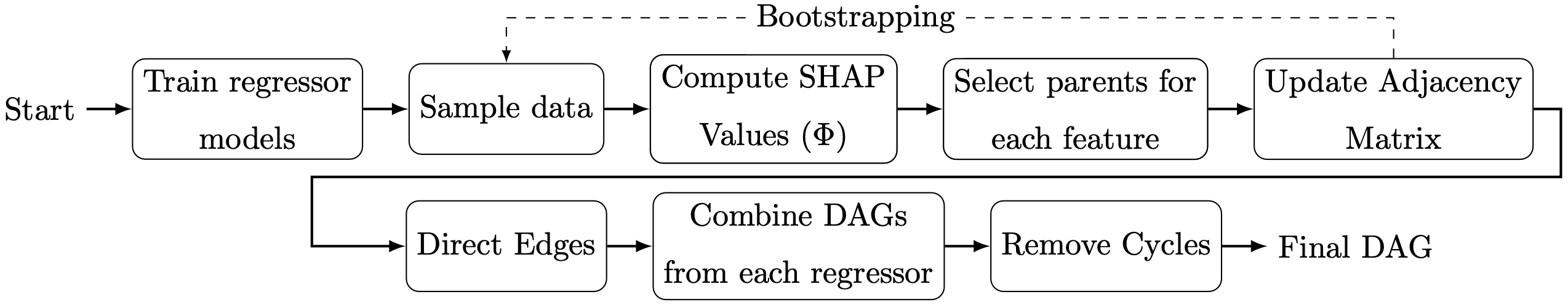
ReX is a causal discovery method that leverages machine learning (ML) models coupled with explainability techniques, specifically Shapley values, to identify and interpret significant causal relationships among variables. Comparative evaluations on synthetic datasets comprising tabular data reveal that ReX outperforms state-of-the-art causal discovery methods across diverse data generation processes, including non-linear and additive noise models. Moreover, ReX was tested on the Sachs single-cell protein-signaling dataset, achieving a precision of 0.952 and recovering key causal relationships with no incorrect edges. Taking together, these results showcase ReX's effectiveness in accurately recovering true causal structures while minimizing false positive predictions, its robustness across diverse datasets, and its applicability to real-world problems. By combining ML and explainability techniques with causal discovery, ReX bridges the gap between predictive modeling and causal inference, offering an effective tool for understanding complex causal structures.
Our experimental results, conducted on five families of synthetic datasets with varying complexity, demonstrate that REX consistently recovers true causal relationships with high precision while minimizing false positives and orientation errors, comparing favorably to existing methods. Additionally, REX was tested on the Sachs single-cell protein-signaling dataset (Sachs et al., 2005), achieving a competitive performance with no false positives and recovering important causal relationships. This further validates the applicability of REX to real-world datasets, highlighting its robustness across different types of data.
Prerequisites without Docker
- Operating System: Linux or macOS
- Environment Manager: PyEnv or Conda
- Programming Language: Python 3.13.11 or higher
- Hardware: CPU (CUDA/MPS optional)
Installation
The project can be installed using pip:
$ pip install causalexplain
What's new in v0.8.0
- Adaptive SHAP sampling with stability checks and new controls like
max_shap_samples; GBT defaults toshap.TreeExplainer. - Parallelization for DNN training and bootstrap runs, plus CLI flags for parallel jobs.
- CUDA/MPS device selection and float32 enforcement for PyTorch models.
- Prior handling and diagnostics improvements across ReX, SHAP, and feature selection.
Data
The datasets used in the paper and the examples can be generated using the
generators module, which is also part of this library. In case you want to
reproduce results from the articles that we used as reference, you can find
the datasets in the data folder.
Executing causalexplain
Option 1: Command Line
To run causalexplain on your data, you can use the causalexplain command:
$ python -m causalexplain --help
   ___                      _                 _       _
  / __\__ _ _   _ ___  __ _| | _____  ___ __ | | __ _(_)_ __
 / /  / _` | | | / __|/ _` | |/ _ \ \/ / '_ \| |/ _` | | '_ \
/ /__| (_| | |_| \__ \ (_| | |  __/>  <| |_) | | (_| | | | | |
\____/\__,_|\__,_|___/\__,_|_|\___/_/\_\ .__/|_|\__,_|_|_| |_|
                                       |_|
usage: causalexplain [-h] [-a | --shap-sampling | --no-shap-sampling]
                     [-b BOOTSTRAP] [-B BOOTSTRAP_PARALLEL_JOBS]
                     [-c {union,intersection}] [-C]
                     [-d DATASET] [-H MAX_SHAP_SAMPLES] [-i ITERATIONS]
                     [-l LOAD_MODEL] [-m {rex,pc,fci,ges,lingam,cam,notears}]
                     [-M] [-n] [-o OUTPUT] [-P PARALLEL_JOBS] [-p PRIOR] [-q]
                     [-s [SAVE_MODEL]] [-S SEED] [-T THRESHOLD] [-t TRUE_DAG]
                     [-v]```

that will present you with a menu to choose the dataset you want to use, the
method you want to use to infer the causal graph, and the hyperparameters you
want to use.

The minimum required to run `causalexplain` is a dataset file in CSV format,
with the first row containing the names of the variables, and the rest of
the rows containing the values of the variables. The method selected by default
is ReX, but you can also choose between PC, FCI, GES, LiNGAM, CAM, NOTEARS.
At the end of the execution, the edges of the plausible causal graph will be
displayed along with the metrics obtained, if the true dag is provided
(argument `-t`).

### Option 2: Notebook

In case you want to run `causalexplain` from your code in a notebook, you can
use the `GraphDiscovery` class. The following example shows how to use
the `GraphDiscovery` class to train a model on a dataset using **ReX** method:

Note: If the notebook kernel cannot import `causalexplain`, run the notebook
from the repo root, or install the package (`pip install -e .`), or add the
repo root to `sys.path` (e.g.: `sys.path.insert(0, str(pathlib.Path("..").resolve()))
`).
For higher-quality math text in plots, install a LaTeX distribution; otherwise
pass `usetex=False` when plotting.
See `examples/simple_experiment.ipynb` for a working notebook example.

```python
from causalexplain import GraphDiscovery

experiment = GraphDiscovery(
   experiment_name='toy_experiment',
   model_type='rex',
   csv_filename='../data/toy_dataset.csv',
   true_dag_filename='../data/toy_dataset.dot')

# Run the experiments
experiment.run(hpo_iterations=10, bootstrap_iterations=10, combine_op='union', quiet=True)

# Plot the resulting DAG (avoid LaTeX/Graphviz dependencies when running locally)
experiment.plot(show_metrics=True, layout='circular', usetex=False)
To load a model from a file, you can use the load method of the
GraphDiscovery class:
from causalexplain import GraphDiscovery

experiment = GraphDiscovery()
experiment.load("/path/to/model.pkl")
Adaptive SHAP sampling
For direct SHAP usage in notebooks, the explainability module exposes a high-level wrapper that defaults to adaptive sampling:
from causalexplain.explainability.shapley import compute_shap

# default: adaptive_shap_sampling=True
res, diag = compute_shap(X, model, backend="kernel", adaptive_shap_sampling=True)

# disable (may be slow for large m)
res, diag = compute_shap(X, model, backend="kernel", adaptive_shap_sampling=False)
CLI example (same executable shown above):
python -m causalexplain --shap-sampling
python -m causalexplain --no-shap-sampling
Available SHAP backends are kernel, gradient, explainer, and tree.
ReX defaults to tree when running the GBT regressor.
When adaptive sampling is enabled, the key knobs are max_shap_samples,
K_max, max_explain_samples, and stratify. These
control background size, repeated sampling for stability, and how many rows
are explained.
Note on large datasets: if adaptive_shap_sampling=False and m > 2000, the
tool warns about potential non-termination (the threshold is conservative).
Why adaptive sampling is mathematically reasonable
Many SHAP explainers approximate an expectation over a background distribution; using $n$ background points gives a Monte Carlo estimate. The standard error scales approximately as $SE \sim \frac{1}{\sqrt{n}}$. So, when sampling without replacement from a finite dataset of size $m$, the finite population correction factor applies: $\frac{1}{\sqrt{1 - (n/m)}}$.
This means increasing $n$ yields diminishing returns, so capping the background around 250 is a pragmatic speed/accuracy tradeoff. Repeating the sampling ($K$ runs) provides a stability diagnostic: compute a global importance vector per run as $\overline{\mid \text{SHAP} \mid}$ per feature, then check variability (CV) and rank stability (Spearman correlation) across runs.
Backend-aware note: Kernel SHAP is particularly sensitive and expensive, so
caps like max_explain_samples matter most there. Gradient and generic
explainers often have different performance profiles, but still benefit from
controlled baselines/background sizes.
This can be useful if you want to train a model on a dataset and then use it to predict causal graphs on other datasets, or train a model on different batches.
Once a model has been trained or loaded, you can plot the resulting DAG, save the trained model to a file, or export the predicted causal graph to a DOT file.
# Plot the resulting DAG
experiment.plot(show_metrics=True, layout='circular', usetex=False)

# Save the trained model to a file
experiment.save("/path/to/model.pkl")
To export the predicted causal graph to a DOT file, you can use the export
method of the GraphDiscovery class:
experiment.export("/path/to/my_predicted_graph.dot")
Output
The output of causalexplain is typically a graph with the edges of the
plausible causal graph and the metrics obtained from the evaluation of the
causal graph against the true DAG. These results are printed to the console,
unless the '-o' option is specified, in which case the DAG is saved to a
file in DOT format. Metrics are printed only if the true DAG is provided.
Example CLI commands
The following command illustrates how to run causalexplain on the toy dataset
using the ReX method:
$ python -m causalexplain -d /path/to/toy_dataset.csv -t /path/to/toy_dataset.dot
The same command can be used to run causalexplain on the toy dataset using the
CAM method:
$ python -m causalexplain -d /path/to/toy_dataset.csv -m cam -t /path/to/toy_dataset.dot
For more information on command line options, run causalexplain -h or go to
the Quickstart
section in the documentation.
Prior knowledge (ReX)
ReX can optionally use prior knowledge to constrain edge directions when you
already know a rough ordering of variables (for example, temporal tiers).
The prior is a JSON file with a single prior key whose value is a list of
tiers; each tier is a list of column names. Variables in earlier tiers may
cause variables in later tiers, but not vice versa. All names must match the
dataset columns, but you can omit variables you have no prior knowledge about.
Example JSON file:
{
  "prior": [
    ["A", "B"],
    ["C", "D"]
  ]
}
Use it from the CLI with -p/--prior (ReX only):
$ python -m causalexplain -d /path/to/data.csv -p /path/to/prior.json
Or from a notebook:
prior = [["A", "B"], ["C", "D"]]
experiment.run(prior=prior, hpo_iterations=10, bootstrap_iterations=10)
Citation
If you use CausalExplain, please cite the software and/or the related publication below.
Software
Renero, J. (2026). CausalExplain (Version 0.8.0). Available at: https://github.com/renero/causalexplain
BibTeX
@software{causalexplain_software,
  author  = {Jesús Renero},
  title   = {CausalExplain},
  version = {0.8.0},
  url     = {https://github.com/renero/causalexplain},
  date    = {2026-01-04}
}
Related Publication
Renero, J., Maestre, R., & Ochoa, I. (2026). ReX: Causal discovery based on machine learning and explainability techniques. Pattern Recognition, 172, 112491. https://doi.org/10.1016/j.patcog.2025.112491
BibTeX
@article{Renero2026ReX,
  author  = {Jesús Renero and Roberto Maestre and Idoia Ochoa},
  title   = {ReX: Causal discovery based on machine learning and explainability techniques},
  journal = {Pattern Recognition},
  volume  = {172},
  pages   = {112491},
  year    = {2026},
  doi     = {10.1016/j.patcog.2025.112491},
  url     = {https://doi.org/10.1016/j.patcog.2025.112491}
}
Release history Release notifications | RSS feed


Download files
Download the file for your platform. If you're not sure which to choose, learn more about installing packages.
Source Distribution
Built Distribution
Filter files by name, interpreter, ABI, and platform.
If you're not sure about the file name format, learn more about wheel file names.
Copy a direct link to the current filters
File details
Details for the file causalexplain-0.8.0.tar.gz.
File metadata
- Download URL: causalexplain-0.8.0.tar.gz
- Upload date:
- Size: 297.4 kB
- Tags: Source
- Uploaded using Trusted Publishing? No
- Uploaded via: twine/6.2.0 CPython/3.10.19
File hashes
| Algorithm | Hash digest | |
|---|---|---|
| SHA256 |
2007a684865c9b170100e33c161ec55d6ab7b334d2939812441a6b0e680366ff
|
|
| MD5 |
d88b58ec51749c24a3d81005ce0837e5
|
|
| BLAKE2b-256 |
a0eecb148161edba3678ab25af4bc0786fa0a3a9df914e98c349e2901c1442e1
|
File details
Details for the file causalexplain-0.8.0-py3-none-any.whl.
File metadata
- Download URL: causalexplain-0.8.0-py3-none-any.whl
- Upload date:
- Size: 269.3 kB
- Tags: Python 3
- Uploaded using Trusted Publishing? No
- Uploaded via: twine/6.2.0 CPython/3.10.19
File hashes
| Algorithm | Hash digest | |
|---|---|---|
| SHA256 |
72bda3652b58d7d1c75959aac4b0803d9a5df23059ba276669f19d805e7ec239
|
|
| MD5 |
e3cd136df1b5bb5b8b56d9b95ab613ab
|
|
| BLAKE2b-256 |
1505b117ae239d9281a5884253fd9397bf0aacb94573b526ed60bb6d46820243
|


