
chassis-sim
English | 简体中文


A lightweight, reproducible workbench for chassis control, observations, and rewards — Ackermann steering, differential drive, and mecanum, with a NumPy core, behind a Gymnasium API.
chassis-sim is for the loop where you change a controller, an observation layout, or one reward term and want to know what happened before your coffee is cold. One process, one robot, one map, explicit seeds, no simulator install. The package is deliberately small; the parts it does implement are specified down to the bit.
It is not an authoritative physics simulator, a contact simulator, or a multi-agent benchmark suite. If you need contact forces, tire models, or thousands of environments on a GPU, use a real physics stack. chassis-sim is the layer where you test the parts that do not need one.
What it is (and is not)
Use it when you want to:
- iterate on a path tracker, a reward function, or an observation layout without rebuilding a simulation stack;
- pin a regression:
reset(seed=...)reproduces the map, the sensor stream, and the trajectory; - teach or demo chassis kinematics with a readable, dependency-light implementation;
- compare reference controllers on a fixed protocol, with the sample-independence check built in.
Skip it when you need:
- authoritative dynamics: suspension, tire slip, load transfer, 3D, or contact-rich interaction;
- a leaderboard: the evaluation harness is for your own baselines, not for ranking the world;
- GPU-scale rollouts: one environment is one Python object on the CPU.
Three boundaries we do not hide:
- Chassis-level kinematics, not wheel-level rigid-body dynamics. The state is
(x, y, θ)and each step integrates a constant twist in closed form. The wheel layer reports steering angles and wheel speeds for logging and downstream control; it never feeds back into the integrator. There is no suspension, no slip, no load transfer, and no 3D. - Collision is a geometric predicate. Rectangle/circle overlap plus optional swept sampling. A collision is a boolean that terminates the episode; there are no contact forces, no friction, and no pushing.
- No GPU and no built-in vectorized batch. Use Gymnasium vector wrappers if you need parallelism; the library itself does not provide a batched simulator.
At a glance
Three chassis, one normalized action interface, finite observation boxes, Gymnasium ids at -v1.
| Gymnasium id | Chassis | Action layout | Default obs | Physical limits (default EnvConfig) |
|---|---|---|---|---|
ChassisSim-Ackermann-v1 |
Ackermann | [steer, speed] |
128 | v ∈ [-0.6, 1.2] m/s, δ ∈ [-0.526, 0.526] rad, ` |
ChassisSim-DiffDrive-v1 |
differential drive | [speed, yaw] |
128 | v ∈ [-1.2, 1.2] m/s, ` |
ChassisSim-Mecanum-v1 |
mecanum | [vx, vy, yaw] |
129 | v_x ∈ [-1.2, 1.2] m/s, ` |
All action spaces are Box(-1, 1, (d,), float32); the chassis maps normalized actions to physical quantities, so you never supply volts, torques, or raw steering angles. The limits above are what env.chassis.describe()["limits"] reports with the default configuration. A different EnvConfig changes the physical mapping and the action semantics together.
3.0.0 is the API-stability line: from this release on the public API follows semantic versioning, and a breaking change requires a major version. chassis_sim.__version__ reports the installed version.
Installation
pip install chassis-sim
pip install "chassis-sim[planning]"
pip install "chassis-sim[viz]"
pip install "chassis-sim[dev]"
Python 3.10+. Core dependencies are numpy>=1.24, gymnasium>=0.29, and pyyaml>=6.0.
planningaddsnumba>=0.60, the first release with NumPy 2 binary wheels, for the Hybrid-A* and Reeds-Shepp scenarios. The core scenes and the defaultdense_staticmap do not need it.vizaddsmatplotlib>=3.7andimageio>=2.28for recording and stills.devaddspytest,pytest-cov,mypy, andtypes-PyYAML.
Quickstart
import chassis_sim as cs

env = cs.make("ackermann", max_steps=200)
obs, info = env.reset(seed=0)
print("observation:", obs.shape, obs.dtype)

for _ in range(3):
    obs, reward, terminated, truncated, info = env.step([0.2, 0.6])
print(
    "step:",
    info["step"],
    "| cte:",
    round(info["cte"], 3),
    "| done:",
    terminated or truncated,
)
observation: (128,) float32
step: 3 | cte: -0.008 | done: False
reset(seed=0) fixes the default scene as well as the robot state. With no seed, every reset() re-rolls the obstacle field of the default dense_static scene — that is the intended behaviour, not a bug. The same seed twice produces the same map:
import hashlib
import json

import chassis_sim as cs


def fingerprint(env):
    shapes = env.unwrapped.bridge.obstacle_shapes()
    blob = json.dumps(shapes, sort_keys=True).encode()
    return len(shapes), hashlib.sha256(blob).hexdigest()[:8]


env = cs.make("ackermann")
for label, kwargs in (
    ("seed=0", {"seed": 0}),
    ("seed=0 again", {"seed": 0}),
    ("no seed", {}),
    ("no seed again", {}),
):
    env.reset(**kwargs)
    count, digest = fingerprint(env)
    print(f"{label:14s} obstacles={count:2d} digest={digest}")
seed=0         obstacles=12 digest=8e794457
seed=0 again   obstacles=12 digest=8e794457
no seed        obstacles=13 digest=1276d1b6
no seed again  obstacles=12 digest=32a57ddd
reset() chooses a scene in this order:
options=if you pass it, verbatim — including{}. Passing{}opts out of both the scenario defaults anddefault_scenario, and lands on the legacy straight fallback.env.default_reset_optionsattached bycs.make(..., scenario=...).EnvConfig.default_scenario(default"dense_static") whenoptions is None, the environment owns its bridge, and nomap_generatoris set.- The legacy straight fallback when
default_scenario=None.
Explicit options are used as given: the environment does not jitter, drop, or re-seed obstacles you supplied yourself.
import numpy as np

import chassis_sim as cs

env = cs.make("ackermann", scenario="corridor")
env.reset(seed=0)
print("scenario obstacles:", len(env.unwrapped.bridge.obstacle_shapes()))

env.reset(seed=0, options={})
print("options={} obstacles:", len(env.unwrapped.bridge.obstacle_shapes()))

env.reset(
    seed=0,
    options={
        "obstacles": [
            {"shape": {"name": "circle", "radius": 0.3}, "state": [3.0, 5.0, 0.0]}
        ],
        "path_waypoints": np.array([[1.0, 5.0, 0.0], [9.0, 5.0, 0.0]]),
    },
)
print("explicit obstacles:", len(env.unwrapped.bridge.obstacle_shapes()))
scenario obstacles: 2
options={} obstacles: 0
explicit obstacles: 1
Gallery
Eleven assets, all regenerated by one command at scenario seed 0:
python examples/gallery.py --out assets
The five clips are 12 fps replays of real closed-loop runs: the controller drives the
env from a seed-0 reset, and the recorded action sequence is then replayed from the
identical reset state, so every clip is reproducible and every clip reaches the goal.
The six stills are the initial state of a scenario (step 0 after reset, chassis
ackermann, no controller) and carry the obstacle field, the reference path, the
body, and the chassis and scenario names in the corner. Each image links to the
full-size file under assets/.
Chassis kinematics — one reference path, one controller
All three chassis drive the same obstacles_sparse path with the same
pure_pursuit controller, so the only thing that changes is the kinematics.
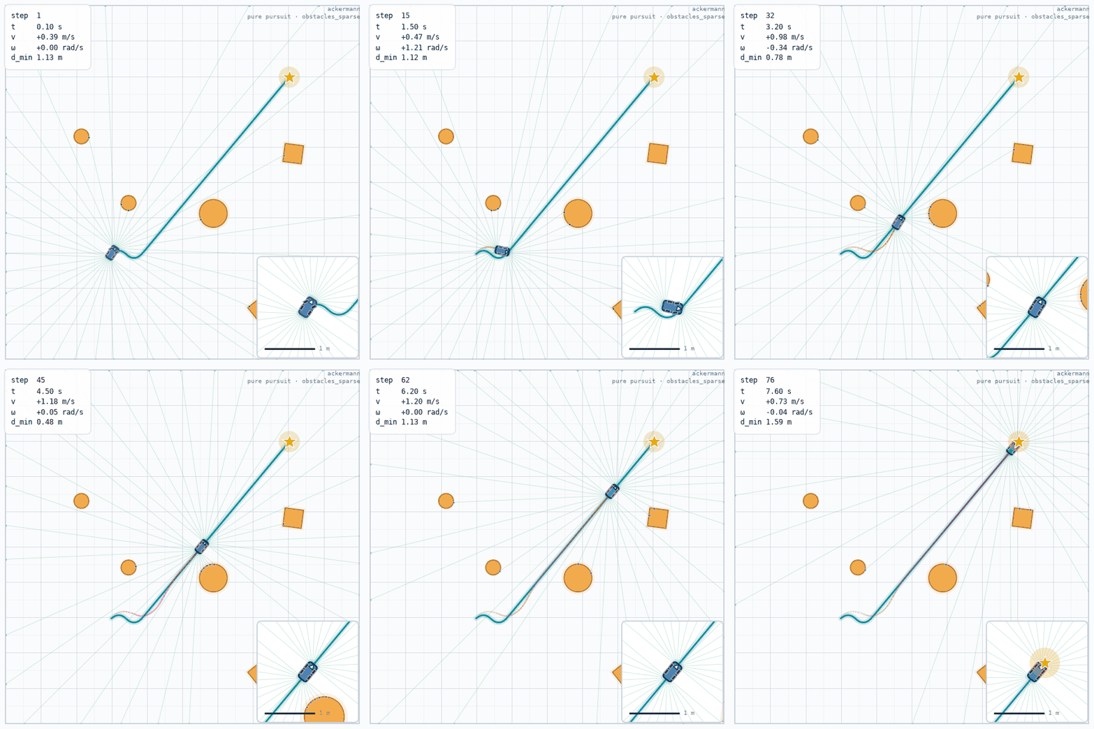 chassis_ackermann.gifobstacles_sparse · ackermann · pure_pursuit |
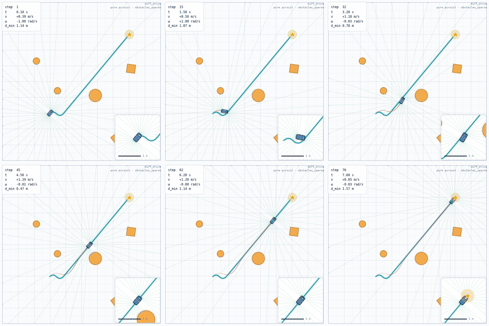 chassis_diff_drive.gifobstacles_sparse · diff_drive · pure_pursuit |
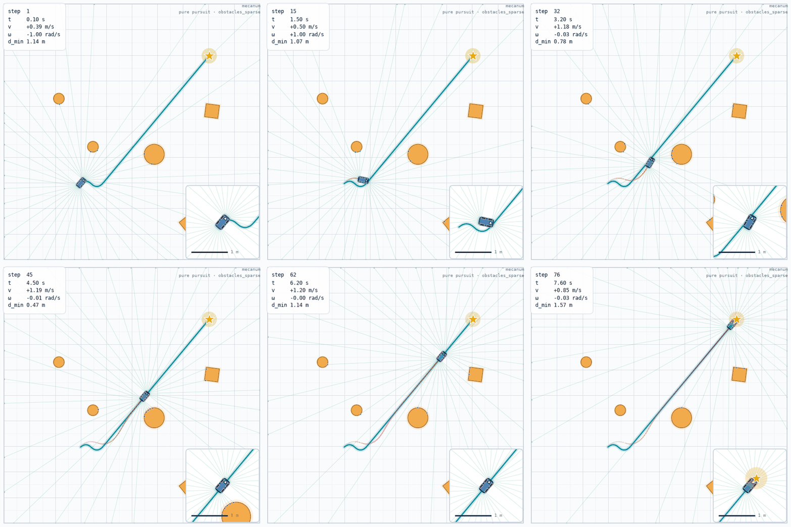 chassis_mecanum.gifobstacles_sparse · mecanum · pure_pursuit |
Front-wheel steering is bounded by the minimum turning radius, so the Ackermann car has to swing wide through a corner. With no lateral degree of freedom the differential-drive turn comes from the wheel-speed difference alone, which reads as a tighter fold on the same path. The mecanum chassis adds the orthogonal velocity component and corrects laterally on the body itself, so it tracks the reference line most closely.
Controllers — one chassis, one scene
Both clips run the ackermann chassis on dense_static, so the difference is the
controller.
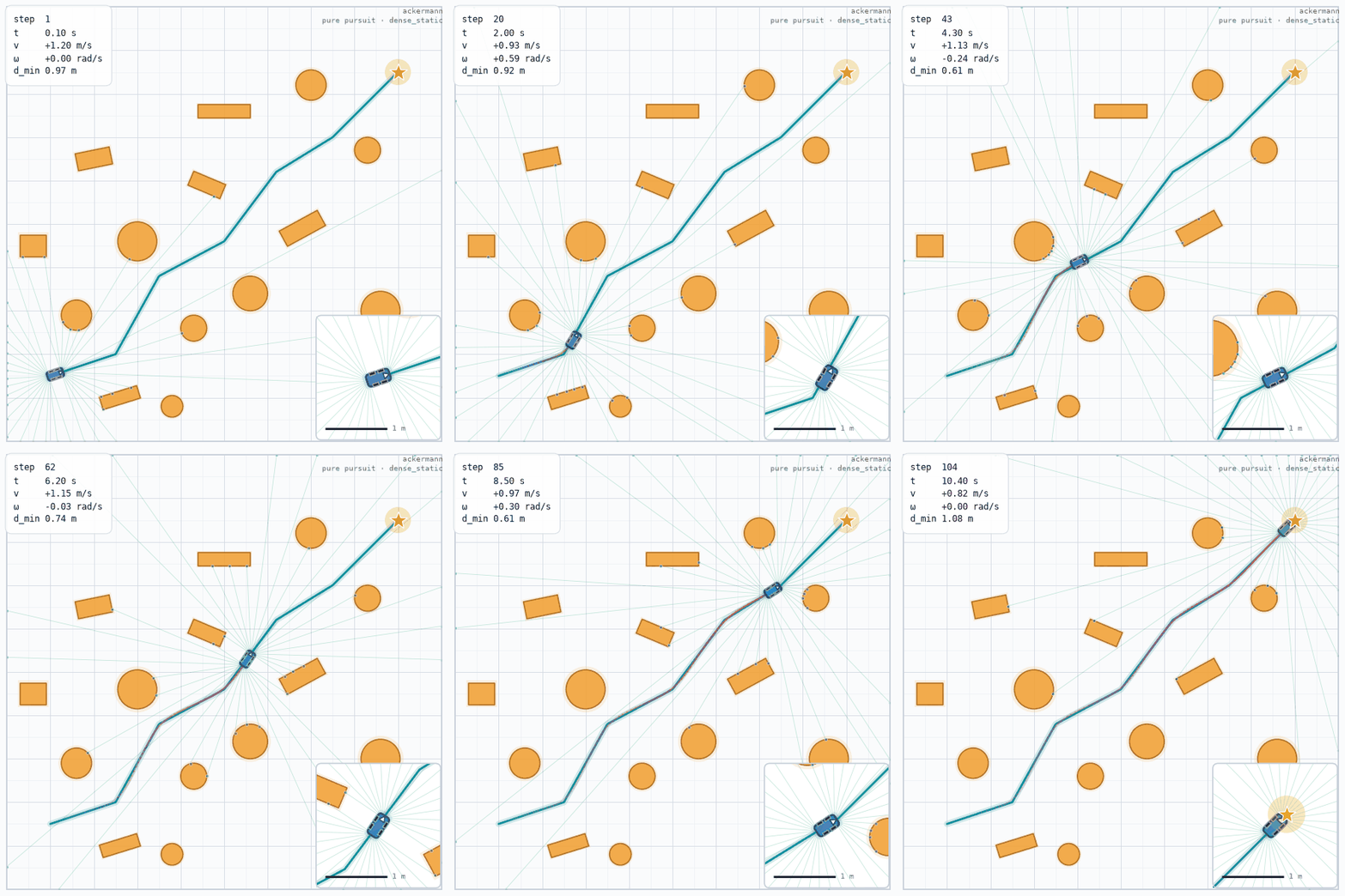 controller_pure_pursuit.gifdense_static · ackermann · pure_pursuit |
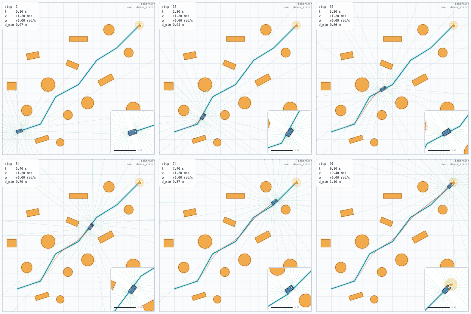 controller_dwa.gifdense_static · ackermann · dwa |
One lookahead arc gives smooth tracking with pure pursuit, but the corners are cut and the body passes closer to the obstacles. Velocity-window sampling plus an obstacle cost makes DWA take the more conservative line and finish in fewer steps.
Scenarios — top-down view
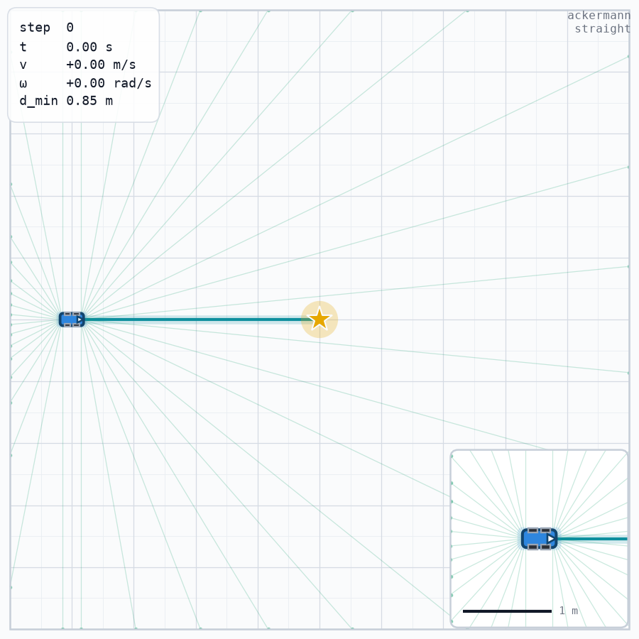 scene_straight.pngstraight · seed 0 · step 0 after reset |
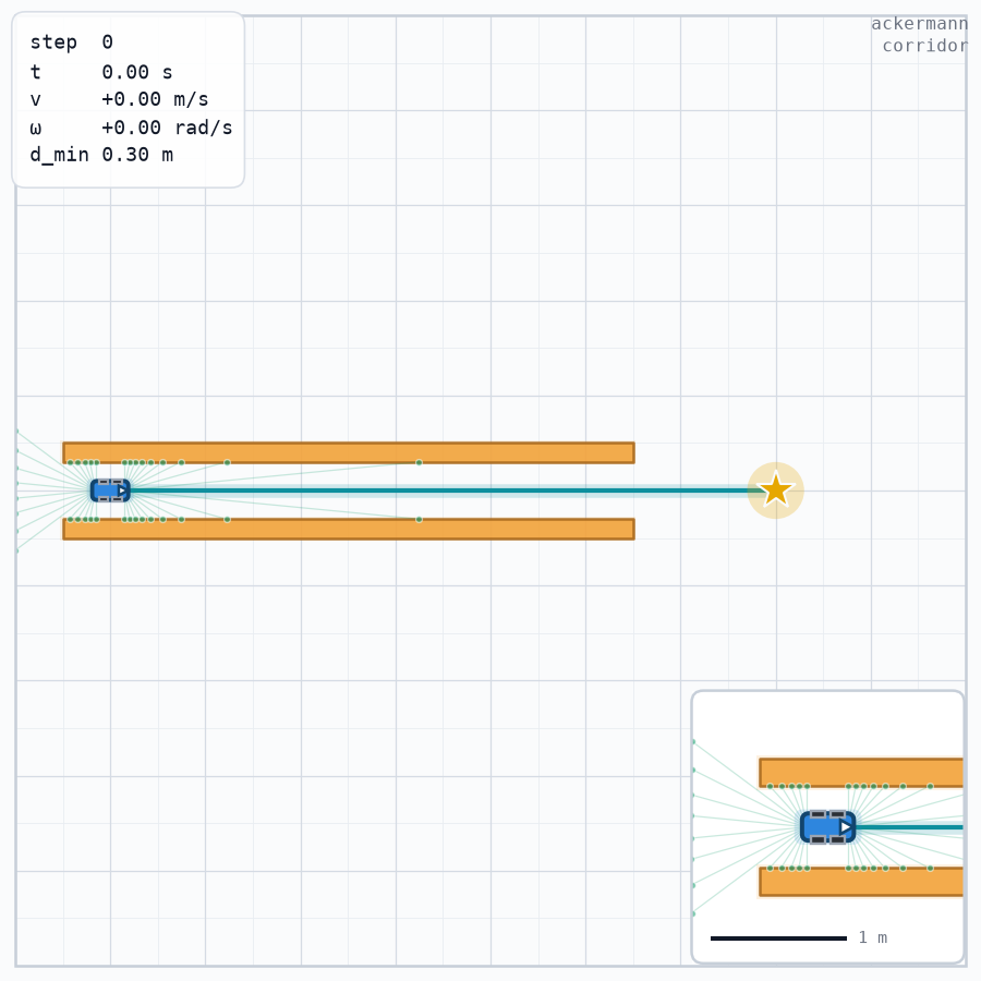 scene_corridor.pngcorridor · seed 0 · step 0 after reset |
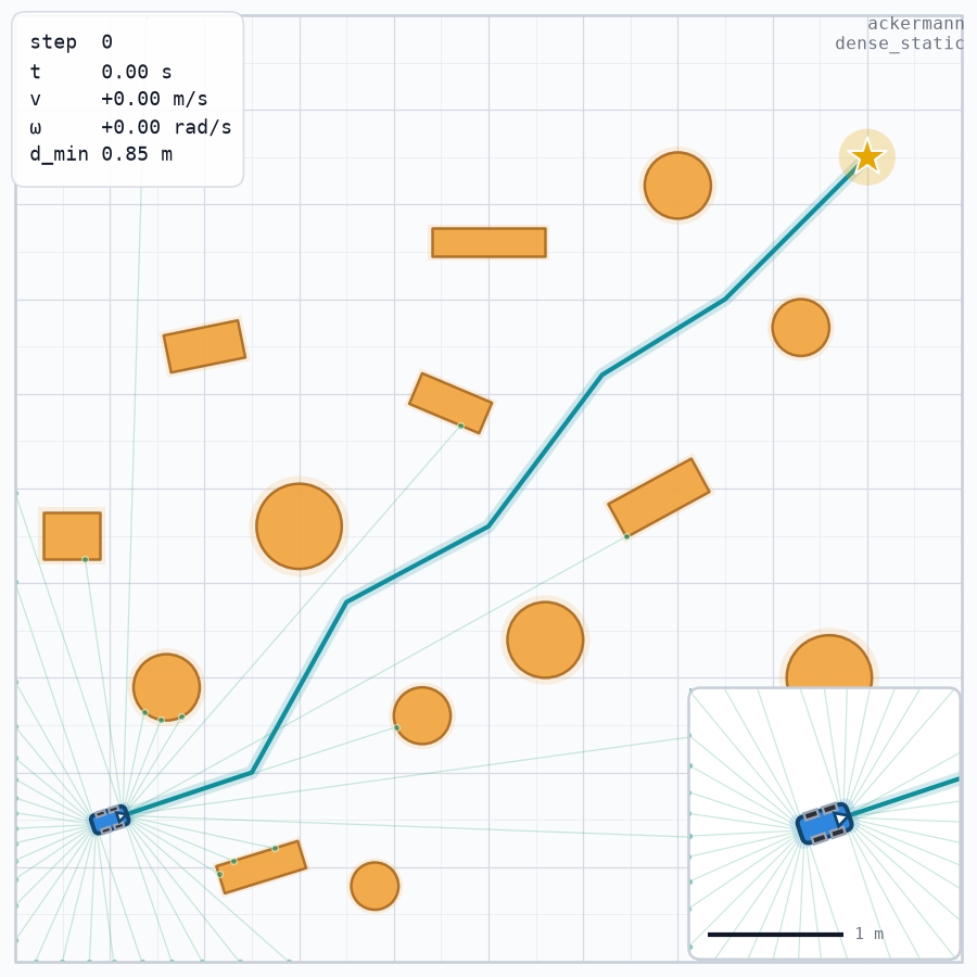 scene_dense_static.pngdense_static · seed 0 · step 0 after reset |
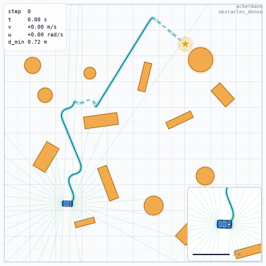 scene_obstacles_dense.pngobstacles_dense · seed 0 · step 0 after reset |
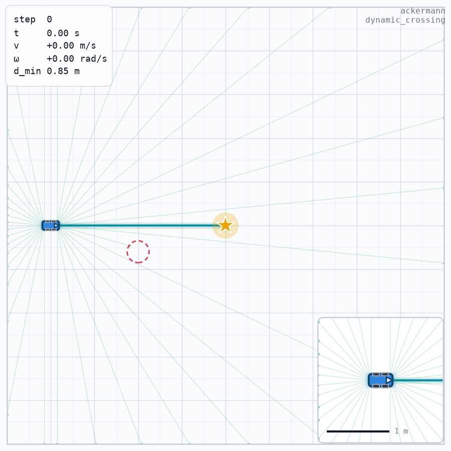 scene_dynamic_crossing.pngdynamic_crossing · seed 0 · step 0 after reset |
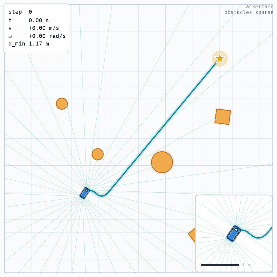 scene_obstacles_sparse.pngobstacles_sparse · seed 0 · step 0 after reset |
straight is the clean baseline: no obstacle, a 4 m reference line at y = 5.
corridor squeezes the feasible region into a 0.6 m band between two long
rectangles, so wall clearance reads off directly. dense_static packs 14 circles
and rectangles against the reference path, hand-written and needing no planner.
obstacles_dense and obstacles_sparse come from the Hybrid-A* map generator, so
their obstacle field is generated per seed rather than stored in YAML: dense draws
9–15 obstacles close to the path, sparse draws 2–5 over open space.
dynamic_crossing has a 0.25 m circle crossing the path at 0.3 m/s on a 20 s
ping-pong cycle, drawn at its t = 0 pose.
Observation and action contract
The observation is a single float32 vector assembled from an ordered list of segments. ObsSpec.default(action_dim, points=30) is four segments — odometry, path, goal, previous action — so it is 128 values wide on the two 2-action chassis and 129 on mecanum.
| Segment | Dim | Contents |
|---|---|---|
Odom |
4 | body-frame [dx*10, dy*10, v, ω] |
PathSegment(points=30) |
120 | per point [ρ, sin φ, cos φ, dθ] — polar, not Cartesian |
Goal |
2 | goal position in the body frame |
Act(action_dim) |
d | previous normalized action |
LidarSegment |
n_rays | scan distances in meters |
Err |
2 | normalized cross-track error and heading error |
GoalSig |
2 | sin and cos of the goal heading error |
PathValid |
1 | 1.0 when the path segment is valid |
PathProgress |
1 | arc completion in [0, 1] |
Custom |
n | your callable |
Every built-in segment declares finite bounds, and observation_space is a finite Box:
world_diagis 14.142 m for the default 10 × 10 m arena; goal coordinates are bounded by it.- Path
ρis bounded byworld_diag + lookahead + 0.1. The default lookahead is 20.0 m, so the upper bound is 34.242 m.sin φandcos φare in[-1, 1];dθis in[-π, π]. - Angle channels are bounded by
π; normalized channels are bounded by1 + 1 ulp= ±1.0000001192092896 after the float32 widening. - Out-of-range values are counted and then clipped.
info["obs_clipped"]is present only when the count is greater than zero; its absence means exactly zero.
import numpy as np

import chassis_sim as cs

env = cs.make("ackermann")
low, high = env.observation_space.low, env.observation_space.high
print("all finite:", bool(np.isfinite(low).all() and np.isfinite(high).all()))
print("path rho:", float(low[4]), "..", round(float(high[4]), 3))
print("normalized channel:", float(high[-1]))
all finite: True
path rho: 0.0 .. 34.242
normalized channel: 1.0000001192092896
Composing your own observation
Segments are composable: adding a lidar, a progress term, or a custom feature is a spec change, not an environment rewrite. The nine-segment, 494-dimension layout is one expression:
import numpy as np

import chassis_sim as cs

env = cs.make(
    "ackermann",
    sensors=[
        cs.Lidar("front", mount=(0.145, 0, 0), n_rays=180),
        cs.Lidar("rear", mount=(-0.155, 0, np.pi), n_rays=180),
    ],
    obs=cs.ObsSpec(
        (
            cs.LidarSegment("lidar", sensors=("front", "rear")),
            cs.Odom(),
            cs.PathSegment(points=30),
            cs.Goal(),
            cs.Act(action_dim=2),
            cs.Err(),
            cs.GoalSig(),
            cs.PathValid(),
            cs.PathProgress(),
        )
    ),
)
print("obs:", env.observation_space.shape)
for name, span in env.obs_spec_describe().items():
    print(f"{name:14s} {span.start:3d}-{span.stop:3d}")
obs: (494,)
lidar            0-360
odom           360-364
path           364-484
goal           484-486
act            486-488
err            488-490
goal_sig       490-492
path_valid     492-493
path_progress  493-494
obs_spec_describe() returns the slice of each segment, so logging and slicing have one source of truth. action_space is Box(-1, 1, (d,), float32); reset() returns (obs, info) and step() returns the five-tuple (obs, reward, terminated, truncated, info).
Sensors
Sensors attach to the bridge and publish readings into info under the sensor name. They do not change the observation unless a LidarSegment references them.
| Sensor | Constructor | info payload |
|---|---|---|
Lidar |
Lidar(name, mount=(x, y, yaw), fov=π, n_rays=180, max_range=10.0, range_min=0.05, noise_std=0, quant_step=0, latency_steps=0, dropout_prob=0) |
scan, scan_meta |
Imu |
Imu(name, noise_std=0) |
ax, ay, yaw_rate, yaw, t |
WheelOdom |
WheelOdom(name, track_width=None, noise_std=0) |
v_left, v_right, v, t |
The default environment has no sensors, and d_min stays at the bridge's max_range (10.0 m) until a lidar provides a nearer hit. Sensor noise is seeded by sensor_seed; when that is unset it falls back to seed, and when both are unset to 0.
import numpy as np

import chassis_sim as cs

env = cs.make(
    "ackermann",
    sensors=[
        cs.Lidar("front", mount=(0.145, 0, 0), n_rays=32, max_range=5.0),
        cs.Imu("imu", noise_std=0.02),
        cs.WheelOdom("wheel", track_width=0.2),
    ],
)
obs, info = env.reset(seed=0)
obs, reward, terminated, truncated, info = env.step(np.zeros(2, dtype=np.float32))
print("scan:", info["front"]["scan"].shape, info["front"]["scan"].dtype)
print("imu keys:", sorted(info["imu"]))
print("wheel keys:", sorted(info["wheel"]))
print("d_min:", round(float(info["d_min"]), 4))
scan: (32,) float32
imu keys: ['ax', 'ay', 't', 'yaw', 'yaw_rate']
wheel keys: ['t', 'v', 'v_left', 'v_right']
d_min: 0.9812
Chassis and wheel kinematics
Each chassis maps normalized actions to a ChassisCommand(v, omega, vy) and integrates a constant twist. A separate, read-only wheel layer reports what the wheels are doing.
| Chassis | Action layout | Command | Wheel kinematics |
|---|---|---|---|
AckermannChassis |
[steer, speed] |
v, ω |
inner and outer front-wheel steering angles |
DiffDriveChassis |
[speed, yaw] |
v, ω |
left and right wheel speeds |
MecanumChassis |
[vx, vy, yaw] |
v, vy, ω |
four wheel angular velocities |
chassis.wheel_kinematics(command) is pure, read-only, and never feeds the integrator. The base class returns None for quantities a chassis does not have — diff drive has no steering angles; mecanum has no left/right pair — rather than an empty dict.
- Ackermann. The front wheels satisfy
cot δ_out − cot δ_in = b / L, withb = 0.2m andL = 0.145m by default. On a left turn the left wheel is the inner one, soδ_left > δ_right. The command[1.0, 0.5]givesδ = 0.526rad,44.03°inner and22.50°outer. - Differential drive.
v_left = v − ω b / 2,v_right = v + ω b / 2. Withv = 1.0,ω = 0.5, andb = 0.2, the wheels turn at 0.95 and 1.05 m/s. - Mecanum. The inverse Jacobian gives
ω_FL = (v − vy − (lx + ly) ω) / r,ω_FR = (v + vy + (lx + ly) ω) / r,ω_RL = (v + vy − (lx + ly) ω) / r,ω_RR = (v − vy + (lx + ly) ω) / r. The forward solution is checked wheel by wheel in the test suite.
import numpy as np

import chassis_sim as cs

ack = cs.AckermannChassis()
command = ack.command(np.array([1.0, 0.5]))
wheels = ack.wheel_kinematics(command)
print(
    "ackermann command: v =", round(command.v, 3), "| omega =", round(command.omega, 3)
)
print(
    "steering (deg):",
    f"{np.degrees(wheels.steering_left):.2f}",
    f"{np.degrees(wheels.steering_right):.2f}",
)

diff = cs.DiffDriveChassis()
wheels = diff.wheel_kinematics(diff.command(np.array([1.0, 0.5])))
print(
    "diff_drive wheels:",
    wheels.wheel_left,
    wheels.wheel_right,
    "| steering:",
    wheels.steering_left,
)

mecanum = cs.MecanumChassis()
wheels = mecanum.wheel_kinematics(mecanum.command(np.array([1.0, 0.5, 0.5])))
print(
    "mecanum wheels:",
    [
        f"{value:.2f}"
        for value in (
            wheels.wheel_fl,
            wheels.wheel_fr,
            wheels.wheel_rl,
            wheels.wheel_rr,
        )
    ],
)
ackermann command: v = 0.5 | omega = 2.0
steering (deg): 44.03 22.50
diff_drive wheels: 0.95 1.05 | steering: None
mecanum wheels: ['12.10', '27.90', '22.10', '17.90']
Controllers
Two reference controllers ship with the package:
| Controller | Defaults | Notes |
|---|---|---|
PurePursuitController |
lookahead=0.6, adaptive=False, lookahead_gain=0.8 |
accepts a path in the body frame |
DwaController |
dt=0.1, horizon=10, gear_mode="off" |
samples the dynamic window |
cs.make_controller("pp"|"dwa", env=env) binds a controller to an environment. A bare PurePursuitController() raises TypeError because the chassis is still unknown; pass env= or chassis=. cs.evaluate(env) with no controller binds pure pursuit for you.
Integration and collision
The state is (x, y, θ). Each step integrates a constant (v, vy, ω) over dt in closed form:
φ = ω dt
A = (sin(θ₀ + φ) − sin θ₀) / ω
B = (cos θ₀ − cos(θ₀ + φ)) / ω
ΔX = v A − vy B
ΔY = v B + vy A
θ = θ₀ + φ
This is the analytic solution, not an approximation. At dt = 0.1, a full circle at v = ω = 1 used to miss its own radius by 5.04e-2 m with the previous Euler step; the closed form's worst radial error over the same circle is 3.33e-16 m.
The branch |ω dt| ≤ sqrt(eps) ≈ 1.49e-8 reproduces the Euler step bit for bit, so ω = 0 trajectories are bitwise identical to the previous implementation (the test suite compares 144 tobytes() pairs).
import math

from chassis_sim.chassis import ChassisCommand, DiffDriveChassis

chassis = DiffDriveChassis(wheelbase=0.145, v_max=1.0, omega_max=1.0)
command = ChassisCommand(v=1.0, omega=1.0)
dt = 0.1
x = y = theta = 0.0
worst = 0.0
for _ in range(round(2 * math.pi / dt)):
    x, y, theta = chassis.integrate(x, y, theta, command, dt)
    worst = max(worst, abs(math.hypot(x, y - 1.0) - 1.0))
print("max radial error:", worst)
max radial error: 3.3306690738754696e-16
Integration substeps
integration_substeps (default 1, validated as an integer ≥ 1) splits each control step into that many closed-form sub-steps. substeps=1 is bitwise identical to the legacy path. With the closed-form integrator, raising it does not improve accuracy — the result is already at float noise (100 steps of a 1 m/s, 1 rad/s arc differ by 9.2e-14 between 1 and 4 sub-steps). What it changes is collision sampling density: more interior poses are tested. Use it for that, not as a "better integrator".
import numpy as np

from chassis_sim.bridges import SimpleBridge
from chassis_sim.chassis import DiffDriveChassis


def pose_after(substeps):
    bridge = SimpleBridge(
        DiffDriveChassis(wheelbase=0.145, v_max=1.0, omega_max=1.0),
        dt=0.1,
        world_bounds=(0, 10, 0, 10),
        domain_rand=False,
        seed=0,
        integration_substeps=substeps,
    )
    bridge.reset(
        path_waypoints=np.array([[1.0, 5.0, 0.0], [9.0, 5.0, 0.0]]),
        initial_heading=0.0,
    )
    for _ in range(100):
        bridge.step(np.array([1.0, 1.0]))
    pose = bridge.pose()
    bridge.close()
    return np.array(pose)


p1, p4 = pose_after(1), pose_after(4)
print("max |substeps=1 - substeps=4|:", float(np.max(np.abs(p1 - p4))))
max |substeps=1 - substeps=4|: 9.237055564881302e-14
Continuous collision detection
ccd (default False) sweep-samples intermediate poses with the same geometric predicate. A 0.1 m wall at 2 m/s — one 2 m step at dt = 0.1 — is missed with CCD off and caught with CCD on:
import numpy as np

from chassis_sim.bridges import SimpleBridge
from chassis_sim.chassis import AckermannChassis


def hits(ccd):
    bridge = SimpleBridge(
        AckermannChassis(v_max=20.0, curvature_action=False),
        dt=0.1,
        world_bounds=(0.0, 10.0, 0.0, 10.0),
        domain_rand=False,
        seed=0,
        ccd=ccd,
    )
    bridge.reset(
        obstacles=[
            {
                "shape": {"name": "rectangle", "length": 0.1, "width": 2.0},
                "state": [1.0, 5.0, 0.0],
            }
        ],
        path_waypoints=np.array([[0.9, 5.0, 0.0], [9.0, 5.0, 0.0]]),
        initial_heading=0.0,
    )
    out = []
    for _ in range(2):
        bridge.step(np.array([0.0, 1.0]))
        out.append(bridge.check_collision())
    bridge.close()
    return out


print("ccd=False:", hits(False))
print("ccd=True: ", hits(True))
ccd=False: [False, False]
ccd=True:  [True, False]
The endpoint test still runs, so the CCD detection set is a superset of the discrete set. Dynamic obstacles are still evaluated at segment ends only.
Evaluation and benchmark
cs.evaluate(env, controller=None, *, episodes, seed=0, max_steps=None, reset_options=None, labels=None, allow_mismatch=False) runs closed-loop episodes and returns an EvalResult with n, successes, collisions, timeouts, the three rates, mean_steps, mean_return, min_obstacle_clearance, success_interval, success_ci, map_fingerprints, distinct_maps, maps_independent, and same_map_repeated.
success_ci is the half-width of a Wilson 95% interval. It is only meaningful when the episodes are independent samples: when distinct_maps < n, the benchmark layer returns None and sets maps_independent=False instead of printing a number computed from repeated maps.
import chassis_sim as cs

env = cs.make("ackermann", max_steps=300)
result = cs.evaluate(env, episodes=10, seed=0)
print(
    "n:",
    result.n,
    "success:",
    f"{result.success_rate:.0%}",
    "steps:",
    f"{result.mean_steps:.1f}",
    "collisions:",
    result.collisions,
)
print(
    "distinct_maps:",
    result.distinct_maps,
    "maps_independent:",
    result.maps_independent,
    "ci:",
    round(result.success_ci, 3),
)
n: 10 success: 100% steps: 102.0 collisions: 0
distinct_maps: 10 maps_independent: True ci: 0.278
Benchmark harness
chassis_sim.eval.benchmark(...) runs the same protocol across policies × scenarios × seeds; python -m chassis_sim benchmark is the command-line entry point. Four baselines ship: zero, random, pp, and dwa.
python -m chassis_sim benchmark \
  --scenarios obstacles_sparse \
  --seeds 0 1 2 \
  --episodes 5 \
  --max-steps 300 \
  --out /tmp/benchmark.md
The cross-seed summary from that run:
| Policy | Success | 95% CI | Collisions | Mean steps | Distinct maps | Independent |
|---|---|---|---|---|---|---|
zero |
0.0% | ±20.4% | 0 | 300.0 | 15 | True |
random |
0.0% | ±20.4% | 6 | 242.8 | 15 | True |
pp |
100.0% | ±20.4% | 0 | 88.9 | 15 | True |
dwa |
100.0% | ±20.4% | 0 | 74.4 | 15 | True |
The interesting column is the last one. Fifteen episodes produced fifteen distinct maps, so the ±20.4% Wilson half-width is a statement about fifteen independent samples. Now run the scenario benchmark uses when --scenarios is omitted:
from chassis_sim.eval import benchmark

result = benchmark(scenarios=["straight"], seeds=[0, 1, 2], episodes=2)
for summary in result.summaries:
    ci = "—" if summary.success_ci is None else f"{summary.success_ci:.1%}"
    print(
        f"{summary.policy:6s} success={summary.success_rate:.0%} ci={ci} "
        f"distinct_maps={summary.distinct_maps} independent={summary.maps_independent}"
    )
zero   success=0% ci=— distinct_maps=1 independent=False
random success=0% ci=— distinct_maps=1 independent=False
pp     success=100% ci=— distinct_maps=1 independent=False
dwa    success=100% ci=— distinct_maps=1 independent=False
straight is a single fixed map. The harness refuses to invent a confidence interval for it: success_ci is None, maps_independent is False, and the markdown output prints —. A table with maps_independent=False is a debugging aid, not a result to quote. benchmark also warns when fewer than three seeds are used and sets protocol_ok=False.
CLI
The package installs a chassis-sim console script; python -m chassis_sim is the same program.
chassis-sim list-scenarios
chassis-sim eval --scenario dense_static --controller pp --episodes 20 --seed 0
chassis-sim record --scenario corridor --controller dwa --out demo.gif --steps 200 --every 4 --fps 12
chassis-sim render --scenario straight --out frame.png --seed 0
python -m chassis_sim benchmark --scenarios obstacles_sparse --seeds 0 1 2 --episodes 5 --max-steps 300 --out -
benchmark --out - prints the table and writes nothing. eval, record, and render default to the planner-free corridor scene; benchmark defaults to straight, which is exactly the repeated-map case above. record and render need the viz extra and exit with status 2 plus a one-line hint when matplotlib or imageio is missing. Planning scenarios need the planning extra and do the same when numba is missing.
Examples
Seven runnable scripts live in examples/. Each one prints what it demonstrates and needs only the extras named above.
| Script | What it shows |
|---|---|
examples/scenario_demo.py |
the three planner-free scenarios driven through cs.make |
examples/sensors_demo.py |
IMU, wheel odometry, and a parameterized LiDAR with latency and dropout |
examples/dynamic_demo.py |
dynamic_crossing: the same open-loop action sequence with static and with moving obstacles |
examples/eval_matrix.py |
the controller × chassis matrix over ten independent maps |
examples/benchmark_baselines.py |
the four baselines rendered as the benchmark table above |
examples/render_demo.py |
an end-to-end render of a planned trajectory in a 10 m × 10 m field |
examples/gallery.py |
the images and GIFs used on this page |
Configuration
EnvConfig is a single dataclass (48 fields) that covers the arena, the chassis, the observation, the sensors, and the default scene. to_yaml() writes a snapshot and from_yaml() reads it back; cs.make(cfg, **overrides) lets explicit keyword arguments win over the config.
import chassis_sim as cs

cfg = cs.EnvConfig(chassis="ackermann", dt=0.1, max_steps=300)
print("fields:", len(cfg.__dataclass_fields__))
print("default_scenario:", cfg.default_scenario)
print("integration_substeps:", cfg.integration_substeps, "| ccd:", cfg.ccd)
path = cfg.to_yaml("/tmp/chassis_sim_env.yaml")
print("first line:", path.read_text().splitlines()[0])
print("roundtrip:", cs.EnvConfig.from_yaml(path) == cfg)
fields: 48
default_scenario: dense_static
integration_substeps: 1 | ccd: False
first line: delta_max: 0.526
roundtrip: True
The fields that matter for the 3.0.0 behaviour are default_scenario, integration_substeps, ccd, seed, and sensor_seed. seed is the run seed used when the env builds its own bridge; reset(seed=...) sets the reset seed explicitly, and sensor_seed falls back to seed when unset.
Scenarios
Eleven scenarios ship as YAML. Core scenes need no extra; planning scenes need numba.
| Scenario | Extra | Obstacles (authored) | Notes |
|---|---|---|---|
straight |
— | 0 | 4 m reference line at y = 5 |
corridor |
— | 2 | 0.6 m band between two long walls |
dense_static |
— | 14 | hand-written default scene |
dynamic_crossing |
— | moving | 0.25 m circle crossing at 0.3 m/s |
circle |
— | 0 | circular reference path |
obstacles_sparse |
planning | 2–5 | Hybrid-A* map |
obstacles_medium |
planning | 5–9 | Hybrid-A* map |
obstacles_dense |
planning | 9–15 | Hybrid-A* map |
obstacles_dense_reverse |
planning | 8–14 | reverse segments |
foldback_reverse |
planning | 10–16 | wide heading range and foldbacks |
maze_grid |
planning | grid | 1.0 m grid, fill ratio 0.4–0.7 |
cs.make(..., scenario=name) attaches that scenario's default_reset_options, so reset(seed=0) uses its fixed map. Passing no scenario gives you the re-rolling dense_static default described in the quickstart. cs.load_scenario(name) returns the parsed Scenario record; a misspelled name raises ScenarioNotFoundError rather than silently falling back. chassis_sim.scenarios.scenario_reset_options_factory(name, base_seed=0) returns a callable that produces a fresh map per episode — the pattern the benchmark uses. Obstacle counts above are what each YAML authors. The dense_static default re-roll applies up to 0.10 m of pose jitter and drops obstacles with probability 0.15 (never below six) on each reset, so its live bridge can expose fewer shapes; scenario defaults and explicit options are used as given.
Rendering
ChassisSimEnv(render_mode=...) accepts None, "human", and "rgb_array". gym.make(id, render_mode=...) and cs.make(..., render_mode=...) pass the mode through. metadata is {"render_modes": ["human", "rgb_array"], "render_fps": 10}; render_fps is derived from dt as max(1, round(1 / dt)), so dt = 0.1 gives 10 fps. After reset(), render() returns a uint8 array of shape (600, 600, 3) for rgb_array and None for human. With render_mode=None, render() warns and returns None rather than silently doing nothing.
import gymnasium as gym

import chassis_sim  # noqa: F401 - importing the package registers the -v1 ids

env = gym.make("ChassisSim-Ackermann-v1", render_mode="rgb_array")
obs, info = env.reset(seed=0)
frame = env.render()
print("frame:", frame.shape, frame.dtype)
print("metadata:", env.metadata)
env.close()
frame: (600, 600, 3) uint8
metadata: {'render_modes': ['human', 'rgb_array'], 'render_fps': 10}
cs.record(env, controller, out="demo.gif", every=4, fps=12) and cs.snapshot(env, "frame.png") live in the viz extra; chassis-sim render writes a single PNG.
Migrating from 2.x
3.0.0 is the API-stability line. The breaking surface from 2.x is exactly three items:
- Gymnasium ids moved from
-v0to-v1. The-v0ids are no longer registered;gym.make("ChassisSim-Ackermann-v0")raisesDeprecatedEnvand names the-v1id to use instead. - The default scene changed.
EnvConfig.default_scenariodefaults to"dense_static", and areset()without an explicit seed re-rolls that map. Setdefault_scenario=Noneto restore the 2.x straight fallback, or passscenario="straight". - The observation space is finite.
observation_spaceis now aBoxwhose low and high are all finite; 2.x advertised an unbounded box. Code that relied on infinite bounds must use the new values (the contract above lists them).
import warnings

import gymnasium as gym

import chassis_sim  # noqa: F401 - importing the package registers the -v1 ids

warnings.filterwarnings("ignore", category=DeprecationWarning)
try:
    gym.make("ChassisSim-Ackermann-v0")
except gym.error.DeprecatedEnv as exc:
    print(f"{type(exc).__name__}: {exc}")
DeprecatedEnv: Environment version v0 for `ChassisSim-Ackermann` is deprecated. Please use `ChassisSim-Ackermann-v1` instead.
Everything else in the 2.x public API keeps working. CHANGELOG.md has the release notes.
License, contributing, and citation
MIT. See LICENSE.
Contributing — the development environment, the exact gates your pull request must pass, and what a reviewable PR looks like — is in CONTRIBUTING.md. Security reports go through the private channel described in SECURITY.md, never a public issue.
Tests and lint:
env -u PYTHONPATH pytest -q
ruff check .
CI runs the test suite on Python 3.10, 3.11, 3.12, and 3.13 (.github/workflows/ci.yml).
If you use this package in academic work, cite the repository — the same metadata is machine-readable in CITATION.cff, which is what GitHub's "Cite this repository" button reads:
@software{chassis_sim_2026,
  author = {ravenkernel},
  title = {chassis-sim: Gymnasium environments for Ackermann, differential-drive
           and mecanum chassis},
  year = {2026},
  url = {https://github.com/ravenkernel/chassis-sim}
}
Every python block in this README is executed as written by tools/check_readme_blocks.py; the text block under each one is that run's stdout. Version numbers name the release line; pyproject.toml remains the single source of truth for the installed version.
1 maintainer

Metadata
1 maintainer
Release files for chassis-sim 3.0.1
For a detailed explanation of source distributions (sdists) and built distributions (wheels), please see the package formats documentation.
Source distribution (sdist)
| File | Size | Uploaded | Provenance | Actions |
|---|---|---|---|---|
| chassis_sim-3.0.1.tar.gz | 523.5 kB | Without provenance | Details for chassis_sim-3.0.1.tar.gz |
Built distribution (wheel)
| File | Interpreter | ABI | Platform | Actions Reset |
|---|---|---|---|---|
| chassis_sim-3.0.1-py3-none-any.whl | Python 3 | none | any | Details for chassis_sim-3.0.1-py3-none-any.whl |
Total release size: 881.1 kB
Release files / chassis_sim-3.0.1.tar.gz
| Download URL | chassis_sim-3.0.1.tar.gz |
|---|---|
| Size | 523.5 kB |
| Tags | Source |
|
SHA-256 checksum How to use checksums |
adf746e2ca69a7d8a529c46222aaf3a9f328d190a15b8f4216737ebd7440e6e6
|
|
BLAKE2b-256 checksum How to use checksums |
32d6c78f4429699c28e49c316af30c6c655ce9ce9a3bcf682abeac288ed950d8
|
| Upload date | |
|
Uploaded using Trusted Publishing? What is trusted publishing? |
No |
| Uploaded via |
twine/7.0.0 CPython/3.12.0
|
Release files / chassis_sim-3.0.1-py3-none-any.whl
| Download URL | chassis_sim-3.0.1-py3-none-any.whl |
|---|---|
| Size | 357.6 kB |
| Tags | Python 3 |
|
SHA-256 checksum How to use checksums |
47d63adff345850933515a67659e109b27cb8f49dae28611b06bbef9b15cdde7
|
|
BLAKE2b-256 checksum How to use checksums |
8aac9616446bf41e88ff9e037719c85a07bd8387031deb5aa2d20ee73930dcc3
|
| Upload date | |
|
Uploaded using Trusted Publishing? What is trusted publishing? |
No |
| Uploaded via |
twine/7.0.0 CPython/3.12.0
|
Security for chassis-sim 3.0.1
Provenance
Provenance describes where a file came from. On PyPI, provenance is shared via attestations, which provide a verifiable record of the build or publishing details. View details, limitations and caveats.
No provenance found
None of the files in this release were uploaded with provenance metadata.
A note on package security
PyPI is a repository for distributing packages, not a service for auditing them. While third-party security researchers and our staff do their best to detect and remove malicious packages, PyPI cannot guarantee the quality, security or suitability of any given package.
To learn more about protecting yourself from malicious actors, visit our package security documentation.














