Python package that implements a Cobweb version of the Global Forest Trade Model

Project description
Cobwood is a Python package designed to analyse global forest products markets.
Key Features:
-
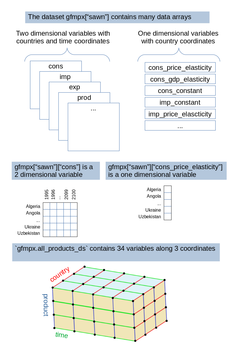
Panel Data Structure: The package represents international forest products market data through 2 dimensional arrays with multiple years and countries, enabling time-series and cross-sectional analysis.
-
Data Handling with Xarray: Utilizes Xarray datasets to efficiently manipulate multi-dimensional data structures. X array is tightly integrated with pandas. Conversion to and from pandas data frames is very straightforward. Xarray datasets are saved on disk using the NetCDF format. This format has the advantage of providing good metadata descriptors. NetCDF is a standard data format used in earth systems modelling, that will just help this model become a component of a greater modelling tool chain.
Documentation
-
The package documentation (generated from function and method docstrings) is available at https://bioeconomy.gitlab.io/cobwood/cobwood/cobwood.html
-
Instructions below explain how to install and run the model. They provide an overview of model formulation and data structure.
-
The paper at paper describes the context and purpose of cobwood.
Installation
Install from the python package index:
pip install cobwood
Install optional development dependencies to run tests or build the documentation:
pip install cobwood[dev]
Input data
The cobwood package requires input data from the cobwood_data repository.
Default data location
By default, cobwood looks for data at ~/repos/cobwood_data/. Clone the repository to
this location:
mkdir -p ~/repos
cd ~/repos
git clone https://gitlab.com/bioeconomy/cobwood/cobwood_data.git
To verify the current data directory location, start python and call:
from cobwood import cobwood_data_dir
print(cobwood_data_dir)
Custom data location (COBWOOD_DATA environment variable)
To use a different location for the data, set the COBWOOD_DATA environment variable
before importing cobwood:
Linux/Mac:
export COBWOOD_DATA="/path/to/your/cobwood_data"
On windows you can set the environment variable in the system GUI, or use a command prompt as follows:
Windows (Command Prompt):
set COBWOOD_DATA=C:\path\to\your\cobwood_data
Windows (PowerShell):
$env:COBWOOD_DATA="C:\path\to\your\cobwood_data"
You can also set it directly in In Python (before importing cobwood):
import os
os.environ["COBWOOD_DATA"] = "/path/to/your/cobwood_data"
from cobwood import cobwood_data_dir
print(cobwood_data_dir)  # Should show your custom path
Then clone the data repository to your chosen location:
mkdir -p /path/to/your/cobwood_data
cd /path/to/your
git clone https://gitlab.com/bioeconomy/cobwood/cobwood_data.git
The input data is based on:
-
A version of the GFPMx model that is no longer available online. More information in the data repository https://gitlab.com/bioeconomy/cobwood/cobwood_data
-
The FAOSTAT forestry production and trade data set available at: http://www.fao.org/faostat/en/#data/FO/visualize
More details in the data repository https://gitlab.com/bioeconomy/cobwood/cobwood_data
Testing
After installing the development dependencies, you can run the test suite to verify the installation and ensure everything works correctly.
Run tests with pytest:
pytest
Doctests are embedded in function docstrings and serve as both documentation and tests. Run doctests through pytest:
pytest --doctest-modules cobwood/
Test coverage
pytest --cov
Type checking
mypy cobwood
Optional virtual environment
Optionally create a virtual environment and install the cobwood package and
its dependencies inside this virtual environment:
mkdir -p /tmp/cobwoodenv
cd /tmp/cobwoodenv/
python3 -m venv /tmp/cobwoodenv/
source /tmp/cobwoodenv/bin/activate
pip install cobwood
Replace /tmp/cobwoodenv with whatever directory path you want to use on your computer.
You can later on use the model inside this virtual environment by activating it each
time with:
source /tmp/cobwoodenv/bin/activate
Run the model
Currently, only the GFFPMx model is available. We will now illustrate how to initiate a model instance for a given scenario. Scenarios are defined in the scenario input directory cobwood_data/scenarios as yaml files. They define variations of the model input, by changing some of the variables, such as the GDP projections for example. Here is how to run the model to reproduce a baseline scenario:
- Load the input data into a GFPMX model object.
from cobwood.gfpmx import GFPMX
gfpmxb2021 = GFPMX(scenario="base_2021", rerun=True)
- Run the model.At each step compare with the reference model run inside the Excel Sheet:
gfpmxb2021.run(compare=True, strict=False)
- Explore the model output tables and make plots.
print(gfpmxb2021["sawn"])
print(gfpmxb2021["sawn"]["cons"])
- Create plots
import matplotlib.pyplot as plt
gfpmxb2021.facet_plot_by_var("indround")
plt.show()
Model Formulation
The core implementation serves as a foundation for developing various versions of global forest sector models. A panel data structure based on N dimensional arrays enable users to extend, or customize the model to fit specific research questions.
The first model formulation is based on GFPMX: "A Cobweb Model of the Global Forest Sector, with an Application to the Impact of the COVID-19 Pandemic" by Joseph Buongiorno https://doi.org/10.3390/su13105507
The GFPMX input data and parameters are available as a spreadsheet at: https://buongiorno.russell.wisc.edu/gfpm/
Equations
Equations are defined using Xarray time and country indexes so that they appear similar
to mathematical equations used in the papers describing the model. For example, the
consumption equation in cobwood/gfpmx_equations.py takes a dataset and a specific time
t as input and returns a data array as output. The input dataset ds contains price
and GDP data for all time steps and all countries, as well as price and GDP
elasticities. The computation at a given time and for a given set of countries is done
by using the time index t and the country index ds.c (which represents all
countries in the dataset) as follows:
def consumption(ds: xarray.Dataset, t: int) -> xarray.DataArray:
    """Compute consumption equation 1"""
    return (
        ds["cons_constant"]
        * pow(ds["price"].loc[ds.c, t - 1], ds["cons_price_elasticity"])
        * pow(ds["gdp"].loc[ds.c, t], ds["cons_gdp_elasticity"])
    )
Data structure
Cobwood implements simulations of the Global Forest Products Market (GFPM), covering data for 180 countries over 80 years. Each equation within the model is structured over two-dimensional Xarray data arrays, where:
- Countries form the first dimension (or coordinate), allowing for cross-sectional analysis.
- Years constitute the second dimension, facilitating time-series insights.
Data Manipulation and Export. Xarray data arrays can be converted to a format
similar to the original GFPMx spreadsheet with countries in rows and years in columns.
For example the following code uses DataArray.to_pandas() to convert the pulp import
array to a csv file using the pandas to_csv() method:
from cobwood.gfpmx_data import GFPMXData
gfpmx_data = GFPMXData(data_dir="gfpmx_8_6_2021", base_year = 2018)
pulp = gfpmx_data.convert_sheets_to_dataset("pulp")
pulp["imp"].to_pandas().to_csv("/tmp/pulp_imp.csv")
Example table containing the first few lines and columns:
| country | 2019 | 2020 | 2021 |
|---|---|---|---|
| Algeria | 66 | 61 | 56 |
| Angola | 0 | 0 | 0 |
| Benin | 0 | 0 | 0 |
The DataArray.to_dataframe() method converts an array and its coordinates into a long
format also called a tidy format with one observation per row.
pulp["imp"].to_dataframe().to_csv("/tmp/pulp_imp_long.csv")
Example table containing the first few lines and columns:
| country | year | imp |
|---|---|---|
| Algeria | 2019 | 66 |
| Algeria | 2020 | 61 |
| Algeria | 2021 | 56 |
License
cobwood is released under the MIT License. Copyright (c) 2024 European Union. See the LICENCE.txt file for the full license text.
Third-party software bundled or depended upon by cobwood is provided under its own license terms, listed in NOTICE.txt.
Release history Release notifications | RSS feed


Download files
Download the file for your platform. If you're not sure which to choose, learn more about installing packages.
Source Distribution
Built Distribution
Filter files by name, interpreter, ABI, and platform.
If you're not sure about the file name format, learn more about wheel file names.
Copy a direct link to the current filters
File details
Details for the file cobwood-0.2.5.tar.gz.
File metadata
- Download URL: cobwood-0.2.5.tar.gz
- Upload date:
- Size: 10.5 MB
- Tags: Source
- Uploaded using Trusted Publishing? No
- Uploaded via: twine/6.1.0 CPython/3.13.5
File hashes
| Algorithm | Hash digest | |
|---|---|---|
| SHA256 |
68ff76142d83deae5c67c753091f86ca4970b99c8f443ff8cf368802a02fbcbd
|
|
| MD5 |
877e537fa377d8f2427043f3171fc5c9
|
|
| BLAKE2b-256 |
72c049db7e1e5039dc3f88d2fb5686cda1df66c565d7e33a6ae04ce2ff27922b
|
File details
Details for the file cobwood-0.2.5-py3-none-any.whl.
File metadata
- Download URL: cobwood-0.2.5-py3-none-any.whl
- Upload date:
- Size: 70.6 kB
- Tags: Python 3
- Uploaded using Trusted Publishing? No
- Uploaded via: twine/6.1.0 CPython/3.13.5
File hashes
| Algorithm | Hash digest | |
|---|---|---|
| SHA256 |
2caa780b645bb7a794b3e9b8e5b49c483d9e6d15631089c3c53dd67059d9bcb7
|
|
| MD5 |
9c9860117bd9f9d5318e968016a83aa6
|
|
| BLAKE2b-256 |
429c61eb91d5190b556a6af3ada0ff242eae8f3ffef575e07dd5ce393619b4ec
|


