conformal-tights 0.3.1

A scikit-learn meta-estimator for computing tight conformal predictions

👖 Conformal Tights

Conformal Tights is a Python package that exports:

• a scikit-learn meta-estimator that adds conformal prediction of coherent quantiles and intervals to any scikit-learn regressor
• a Darts forecaster that adds conformally calibrated probabilistic time series forecasting to any scikit-learn regressor

Features

1. 🍬 Sklearn meta-estimator: add conformal prediction of quantiles and intervals to any scikit-learn regressor
2. 🔮 Darts forecaster: add conformally calibrated probabilistic forecasting to any scikit-learn regressor
3. 🌡️ Conformally calibrated: accurate quantiles, and intervals with reliable coverage
4. 🚦 Coherent quantiles: quantiles increase monotonically instead of crossing each other
5. 👖 Tight quantiles: selects the lowest dispersion that provides the desired coverage
6. 🎁 Data efficient: requires only a small number of calibration examples to fit
7. 🐼 Pandas support: optionally predict on DataFrames and receive DataFrame output

Using

Quick links

1. Installing
2. Predicting quantiles
3. Predicting intervals
4. Forecasting time series

Installing

pip install conformal-tights

Predicting quantiles

Conformal Tights exports a meta-estimator called ConformalCoherentQuantileRegressor that you can use to equip any scikit-learn regressor with a predict_quantiles method that predicts conformally calibrated quantiles. Example usage:

from conformal_tights import ConformalCoherentQuantileRegressor
from sklearn.datasets import fetch_openml
from sklearn.model_selection import train_test_split
from xgboost import XGBRegressor

# Fetch dataset and split in train and test
X, y = fetch_openml("ames_housing", version=1, return_X_y=True, as_frame=True, parser="auto")
X_train, X_test, y_train, y_test = train_test_split(X, y, test_size=0.15, random_state=42)

# Create a regressor, equip it with conformal prediction, and fit on the train set
my_regressor = XGBRegressor(objective="reg:absoluteerror")
conformal_predictor = ConformalCoherentQuantileRegressor(estimator=my_regressor)
conformal_predictor.fit(X_train, y_train)

# Predict with the underlying regressor
ŷ_test = conformal_predictor.predict(X_test)

# Predict quantiles with the conformal predictor
ŷ_test_quantiles = conformal_predictor.predict_quantiles(
    X_test, quantiles=(0.025, 0.05, 0.1, 0.9, 0.95, 0.975)
)

When the input data is a pandas DataFrame, the output is also a pandas DataFrame. For example, printing the head of ŷ_test_quantiles yields:

house_id	0.025	0.05	0.1	0.9	0.95	0.975
1357	114784.0	120894.3	131618.0	175760.5	188052.0	205448.8
2367	67416.6	80073.7	86754.0	117854.1	127582.6	142321.9
2822	119422.7	132047.7	138724.6	178526.0	197246.2	214205.6
2126	94030.6	99850.0	110891.3	150249.2	164703.0	182528.1
1544	68996.2	81516.3	88231.6	121774.2	132425.1	147110.2

Let's visualize the predicted quantiles on the test set:

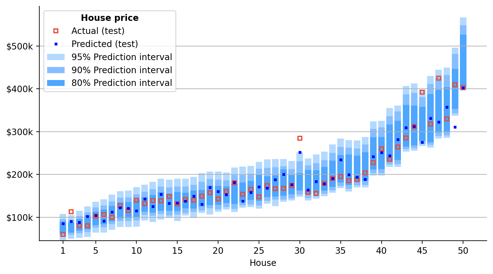
Expand to see the code that generated the graph above

import matplotlib.pyplot as plt
import matplotlib.ticker as ticker

%config InlineBackend.figure_format = "retina"
plt.rc("font", family="DejaVu Sans", size=10)
plt.figure(figsize=(8, 4.5))
idx = ŷ_test.sample(50, random_state=42).sort_values().index
x = list(range(1, len(idx) + 1))
x_ticks = [1, *list(range(5, len(idx) + 1, 5))]
for j in range(3):
    coverage = round(100 * (ŷ_test_quantiles.columns[-(j + 1)] - ŷ_test_quantiles.columns[j]))
    plt.bar(
        x,
        ŷ_test_quantiles.loc[idx].iloc[:, -(j + 1)] - ŷ_test_quantiles.loc[idx].iloc[:, j],
        bottom=ŷ_test_quantiles.loc[idx].iloc[:, j],
        color=["#b3d9ff", "#86bfff", "#4da6ff"][j],
        label=f"{coverage}% Prediction interval",
    )
plt.plot(
    x,
    y_test.loc[idx],
    "s",
    label="Actual (test)",
    markeredgecolor="#e74c3c",
    markeredgewidth=1.414,
    markerfacecolor="none",
    markersize=4,
)
plt.plot(x, ŷ_test.loc[idx], "s", color="blue", label="Predicted (test)", markersize=2)
plt.xlabel("House")
plt.xticks(x_ticks, x_ticks)
plt.gca().yaxis.set_major_formatter(ticker.FuncFormatter(lambda x, _: f"${x/1000:,.0f}k"))
plt.gca().tick_params(axis="both", labelsize=10)
plt.gca().spines["top"].set_visible(False)
plt.gca().spines["right"].set_visible(False)
plt.grid(False)
plt.grid(axis="y")
plt.legend(loc="upper left", title="House price", title_fontproperties={"weight": "bold"})
plt.tight_layout()

Predicting intervals

In addition to quantile prediction, you can use predict_interval to predict conformally calibrated prediction intervals. Compared to quantiles, these focus on reliable coverage over quantile accuracy. Example usage:

# Predict an interval for each example with the conformal predictor
ŷ_test_interval = conformal_predictor.predict_interval(X_test, coverage=0.95)

# Measure the coverage of the prediction intervals on the test set
coverage = ((ŷ_test_interval.iloc[:, 0] <= y_test) & (y_test <= ŷ_test_interval.iloc[:, 1])).mean()
print(coverage)  # 96.6%

When the input data is a pandas DataFrame, the output is also a pandas DataFrame. For example, printing the head of ŷ_test_interval yields:

house_id	0.025	0.975
1357	107202.8	206290.4
2367	66665.1	146004.8
2822	115591.8	220314.8
2126	85288.1	183037.8
1544	67889.9	150646.2

Forecasting time series

Conformal Tights also exports a Darts forecaster called DartsForecaster that uses a ConformalCoherentQuantileRegressor to make conformally calibrated probabilistic time series forecasts. To demonstrate its usage, let's begin by loading a time series dataset:

from darts.datasets import ElectricityConsumptionZurichDataset

# Load a forecasting dataset
ts = ElectricityConsumptionZurichDataset().load()
ts = ts.resample("h")

# Split the dataset into covariates X and target y
X = ts.drop_columns(["Value_NE5", "Value_NE7"])
y = ts["Value_NE5"]  # NE5 = Household energy consumption

# Add categorical covariates to X
X = X.add_holidays(country_code="CH")
X = X.add_datetime_attribute("month")
X = X.add_datetime_attribute("dayofweek")
X = X.add_datetime_attribute("hour")
X_categoricals = ["holidays", "month", "dayofweek", "hour"]

Printing the tail of the covariates time series X.pd_dataframe() yields:

Timestamp	Hr [%Hr]	RainDur [min]	StrGlo [W/m2]	T [°C]	WD [°]	WVs [m/s]	WVv [m/s]	p [hPa]	holidays	month	dayofweek	hour
2022‑08‑30 20h	70.2	0.0	0.0	19.9	290.2	1.7	1.5	968.5	0.0	7.0	1.0	20.0
2022‑08‑30 21h	70.1	0.0	0.0	19.5	239.2	1.0	0.7	968.1	0.0	7.0	1.0	21.0
2022‑08‑30 22h	71.3	0.0	0.0	19.5	28.9	1.5	1.3	967.9	0.0	7.0	1.0	22.0
2022‑08‑30 23h	80.4	0.0	0.0	18.9	24.3	1.6	1.1	967.9	0.0	7.0	1.0	23.0
2022‑08‑31 00h	81.6	1.0	0.0	18.7	293.5	0.9	0.3	967.8	0.0	7.0	2.0	0.0

We can now equip a scikit-learn regressor with conformal prediction using ConformalCoherentQuantileRegressor as before, and then equip that conformal predictor with probabilistic time series forecasting using DartsForecaster:

from conformal_tights import DartsForecaster, ConformalCoherentQuantileRegressor
from pandas import Timestamp
from xgboost import XGBRegressor

# Split the dataset into train and test
test_cutoff = Timestamp("2022-06-01")
y_train, y_test = y.split_after(test_cutoff)
X_train, X_test = X.split_after(test_cutoff)

# Now let's:
# 1. Create an sklearn regressor of our choosing, in this case `XGBRegressor`
# 2. Add conformal quantile prediction to the regressor with `ConformalCoherentQuantileRegressor`
# 3. Add probabilistic forecasting to the conformal predictor with `DartsForecaster`
my_regressor = XGBRegressor()
conformal_predictor = ConformalCoherentQuantileRegressor(estimator=my_regressor)
forecaster = DartsForecaster(
    model=conformal_predictor,
    lags=5 * 24,  # Add the last 5 days of the target to the prediction features
    lags_future_covariates=[0],  # Add the current timestamp's covariates to the prediction features
    categorical_future_covariates=X_categoricals,  # Convert these covariates to pd.Categorical
)

# Fit the forecaster
forecaster.fit(y_train, future_covariates=X_train)

# Make a probabilistic forecast 5 days into the future by predicting a set of conformally calibrated
# quantiles at each time step and drawing 500 samples from them
quantiles = (0.025, 0.05, 0.1, 0.25, 0.5, 0.75, 0.9, 0.95, 0.975)
forecast = forecaster.predict(
    n=5 * 24, future_covariates=X_test, num_samples=500, quantiles=quantiles
)

Printing the head of the forecast quantiles time series forecast.quantiles_df(quantiles=quantiles) yields:

Timestamp	Value_NE5_0.025	Value_NE5_0.05	Value_NE5_0.1	Value_NE5_0.25	Value_NE5_0.5	Value_NE5_0.75	Value_NE5_0.9	Value_NE5_0.95	Value_NE5_0.975
2022‑06‑01 01h	19197.4	19262.5	19366.4	19612.7	19786.7	19996.5	20185.5	20293.3	20358.0
2022‑06‑01 02h	18963.2	19078.7	19263.3	19463.6	19706.0	19951.4	20125.2	20265.8	20353.4
2022‑06‑01 03h	19259.1	19372.3	19551.2	19846.4	20145.2	20401.1	20630.4	20814.0	20939.6
2022‑06‑01 04h	21537.8	21745.9	21958.0	22266.8	22600.7	22939.7	23356.0	23538.7	23691.7
2022‑06‑01 05h	24304.0	24503.6	24717.5	25029.4	25602.3	26266.4	26791.6	26963.8	27359.2

Let's visualize the forecast and its prediction interval on the test set:

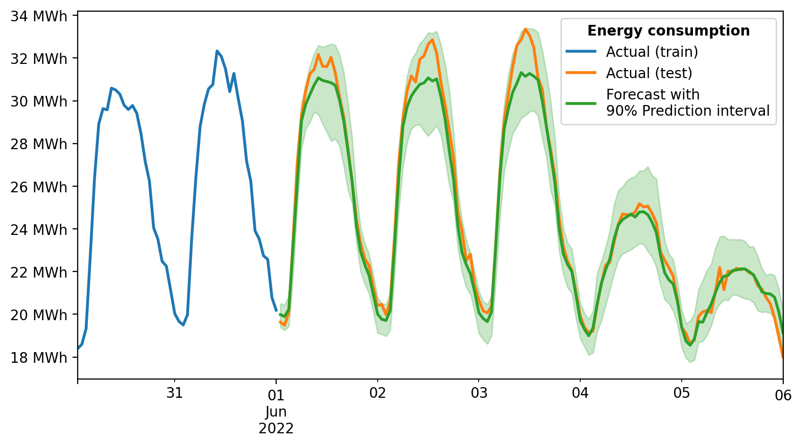
Expand to see the code that generated the graph above

import matplotlib.pyplot as plt
import matplotlib.ticker as ticker

%config InlineBackend.figure_format = "retina"
plt.rc("font", family="DejaVu Sans", size=10)
plt.figure(figsize=(8, 4.5))
y_train[-2 * 24 :].plot(label="Actual (train)")
y_test[: len(forecast)].plot(label="Actual (test)")
forecast.plot(label="Forecast with\n90% Prediction interval", low_quantile=0.05, high_quantile=0.95)
plt.gca().set_xlabel("")
plt.gca().yaxis.set_major_formatter(ticker.FuncFormatter(lambda x, _: f"{x/1000:,.0f} MWh"))
plt.gca().tick_params(axis="both", labelsize=10)
plt.legend(loc="upper right", title="Energy consumption", title_fontproperties={"weight": "bold"})
plt.tight_layout()

Contributing

Prerequisites

1. Set up Git to use SSH

1. Generate an SSH key and add the SSH key to your GitHub account.

2. Configure SSH to automatically load your SSH keys:

   cat << EOF >> ~/.ssh/config
   Host *
     AddKeysToAgent yes
     IgnoreUnknown UseKeychain
     UseKeychain yes
   EOF
   

2. Install Docker

1. Install Docker Desktop.
   • Enable Use Docker Compose V2 in Docker Desktop's preferences window.
   • Linux only:

     • Export your user's user id and group id so that files created in the Dev Container are owned by your user:

       cat << EOF >> ~/.bashrc
       export UID=$(id --user)
       export GID=$(id --group)
       EOF
       

3. Install VS Code or PyCharm

1. Install VS Code and VS Code's Dev Containers extension. Alternatively, install PyCharm.
2. Optional: install a Nerd Font such as FiraCode Nerd Font and configure VS Code or configure PyCharm to use it.

Development environments

The following development environments are supported:

1. ⭐️ GitHub Codespaces: click on Code and select Create codespace to start a Dev Container with GitHub Codespaces.
2. ⭐️ Dev Container (with container volume): click on Open in Dev Containers to clone this repository in a container volume and create a Dev Container with VS Code.
3. Dev Container: clone this repository, open it with VS Code, and run Ctrl/⌘ + ⇧ + P → Dev Containers: Reopen in Container.
4. PyCharm: clone this repository, open it with PyCharm, and configure Docker Compose as a remote interpreter with the dev service.
5. Terminal: clone this repository, open it with your terminal, and run docker compose up --detach dev to start a Dev Container in the background, and then run docker compose exec dev zsh to open a shell prompt in the Dev Container.

Developing

• This project follows the Conventional Commits standard to automate Semantic Versioning and Keep A Changelog with Commitizen.
• Run poe from within the development environment to print a list of Poe the Poet tasks available to run on this project.
• Run poetry add {package} from within the development environment to install a run time dependency and add it to pyproject.toml and poetry.lock. Add --group test or --group dev to install a CI or development dependency, respectively.
• Run poetry update from within the development environment to upgrade all dependencies to the latest versions allowed by pyproject.toml.
• Run cz bump to bump the package's version, update the CHANGELOG.md, and create a git tag.