Plotting tools for complex-valued functions

Project description

Plot complex-valued functions with style.


cplot helps plotting complex-valued functions in a visually appealing manner. The general idea is to map the absolute value to lightness and the complex argument (the "angle") to the chroma of the representing color. This follows the domain coloring approach, also described by John D. Cook and Elias Wegert in the book Visual Complex Functions (with some tweaks). Also check out the DC gallery by Juan Carlos Ponce Campuzano.
Similar projects:
Install with
pip install cplot
and use as
import cplot
import numpy
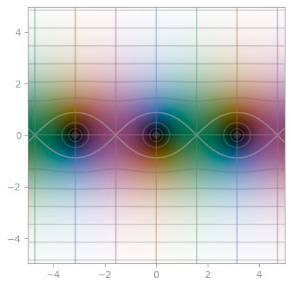
cplot.show(numpy.tan, -5, +5, -5, +5, 100, 100)
cplot.save_fig("out.png", numpy.tan, -5, +5, -5, +5, 100, 100)
cplot.save_img("out.png", numpy.tan, -5, +5, -5, +5, 100, 100)
# There is a tripcolor function as well for triangulated 2D domains
# cplot.tripcolor(triang, z)
# The function get_srgb1 returns the SRGB1 triple for every complex input value.
# (Accepts arrays, too.)
z = 2 + 5j
val = cplot.get_srgb1(z)
All functions have the optional arguments (with their default values)
alpha=1  # >= 0
colorspace="cam16"  # "cielab", "hsl"
-
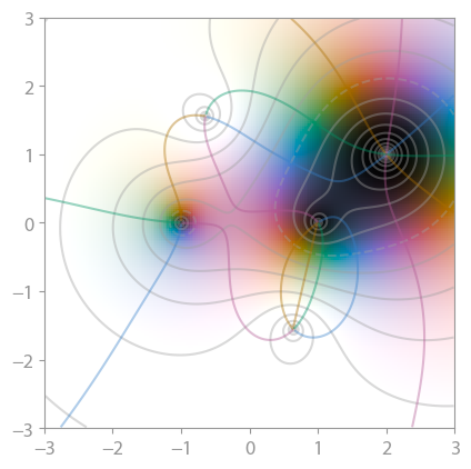
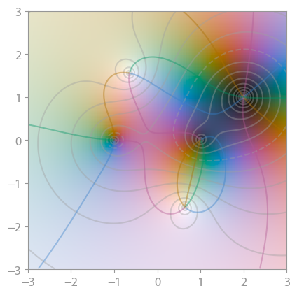
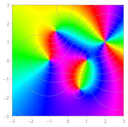
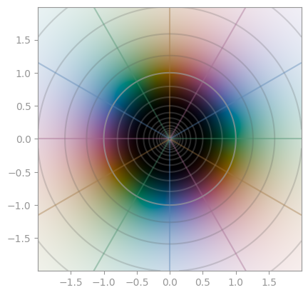
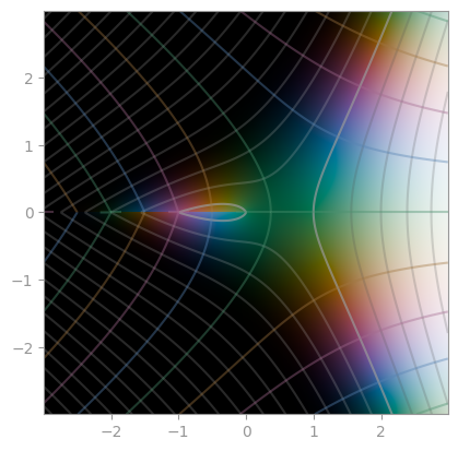
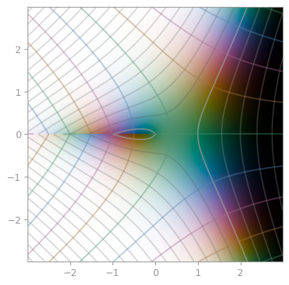
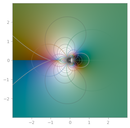
alphacan be used to adjust the use of colors. A value less than 1 adds more color which can help isolating the roots and poles (which are still black and white, respectively).alpha=0ignores the magnitude off(z)completely. -
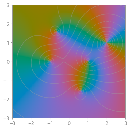
colorspacecan be set tohslto get the common fully saturated, vibrant colors. This is usually a bad idea since it creates artifacts which are not related with the underlying data. From Wikipedia:Since the HSL color space is not perceptually uniform, one can see streaks of perceived brightness at yellow, cyan, and magenta (even though their absolute values are the same as red, green, and blue) and a halo around L = 1 / 2 . Use of the Lab color space corrects this, making the images more accurate, but also makes them more drab/pastel.
Default is
"cam16"; very similar is"cielab"(not shown here).
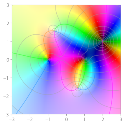
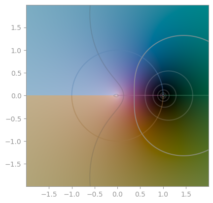
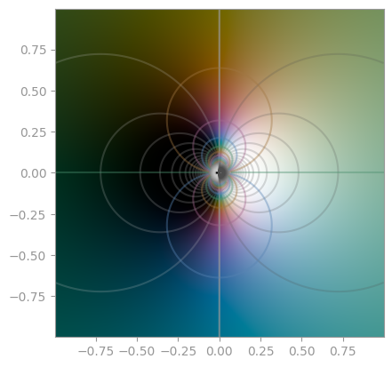
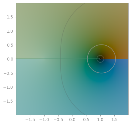
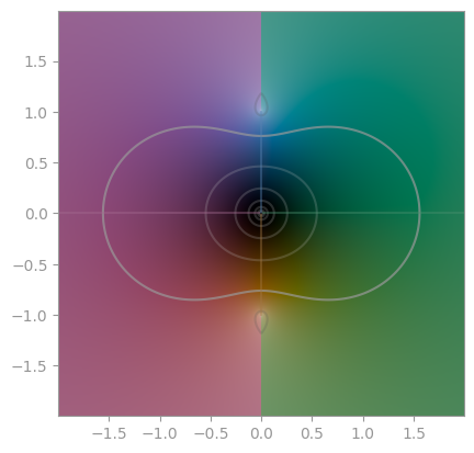
Consider the test function (z ** 2 - 1) * (z - 2 - 1j) ** 2 / (z ** 2 + 2 + 2j):
alpha = 1 |
alpha = 0.5 |
alpha = 0.0 |
|---|---|---|
 |
 |
 |
 |
 |
 |
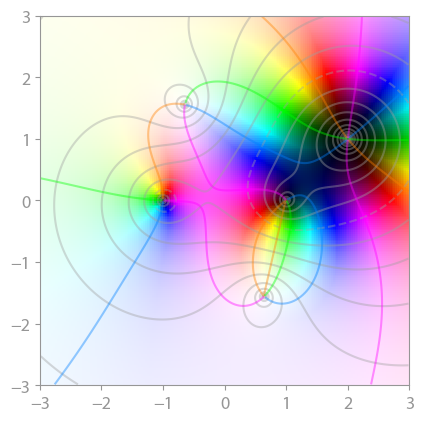
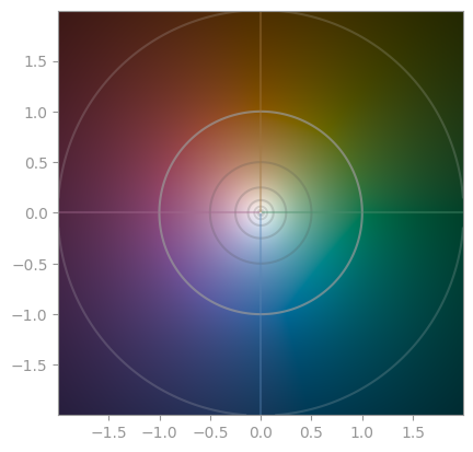
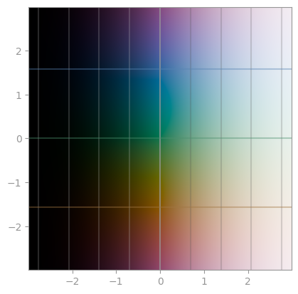
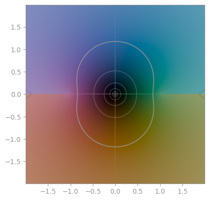
The representation is chosen such that
- values around 0 are black,
- values around infinity are white,
- values around +1 are green,
- values around -1 are deep purple,
- values around +i are blue,
- values around -i are orange.
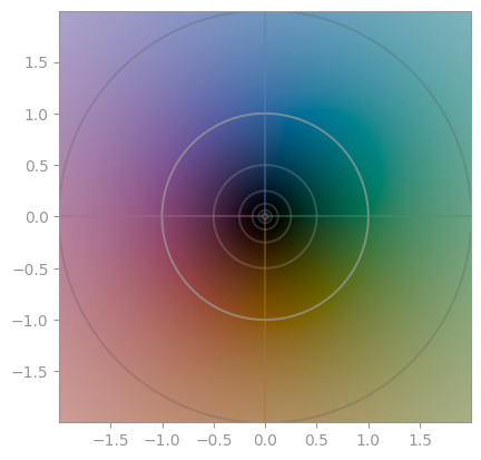
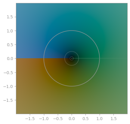
(Compare to the z1 reference plot below.)
With this, it is easy to see where a function has very small and very large values, and the multiplicty of zeros and poles is instantly identified by counting the color wheel passes around a black or white point.
Gallery
All plots are created with default settings.
 |
 |
 |
|---|---|---|
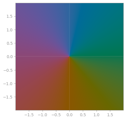
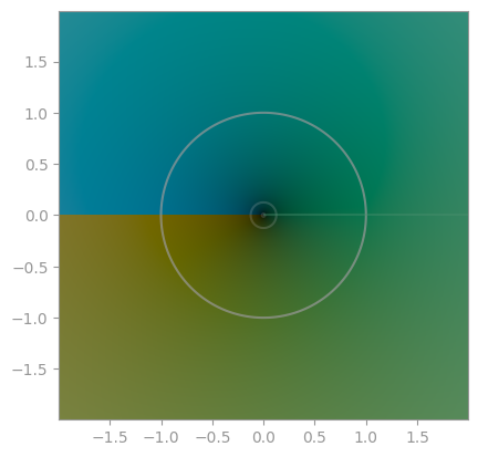
z**1 |
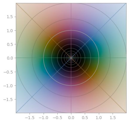
z**2 |
z**3 |
 |
 |
 |
|---|---|---|
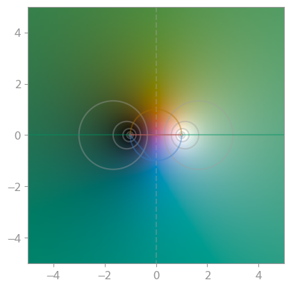
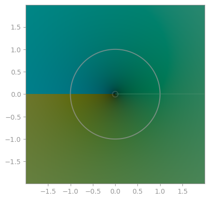
1/z |
z / abs(z) |
(z+1) / (z-1) |
 |
 |
 |
|---|---|---|
z ** z |
(1/z) ** z |
z ** (1/z) |
 |
 |
 |
|---|---|---|
numpy.sqrt |
z**(1/3) |
z**(1/4) |
 |
 |
 |
|---|---|---|
numpy.log |
numpy.exp |
exp(1/z) |
 |
 |
 |
|---|---|---|
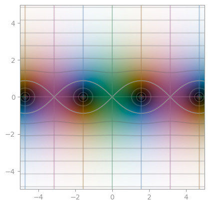
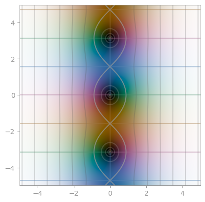
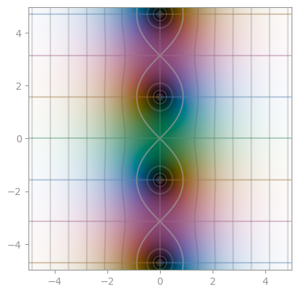
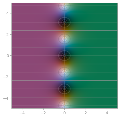
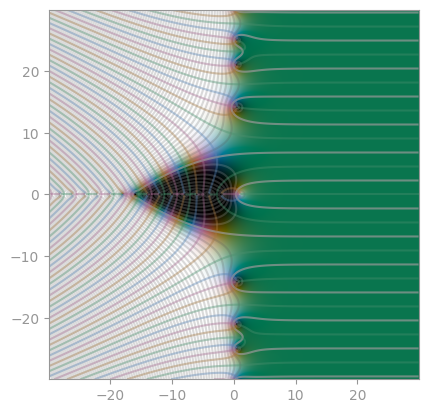
numpy.sin |
numpy.cos |
numpy.tan |
 |
 |
 |
|---|---|---|
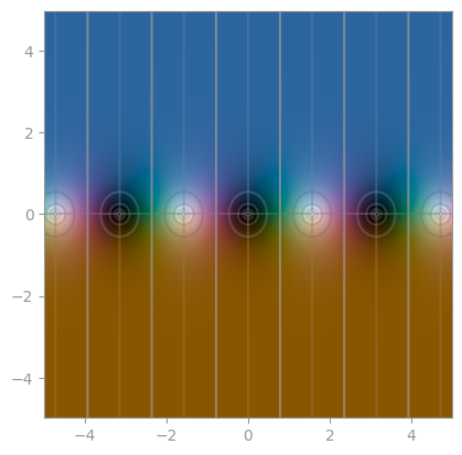
numpy.sinh |
numpy.cosh |
numpy.tanh |
 |
 |
 |
|---|---|---|
numpy.arcsin |
numpy.arccos |
numpy.arctan |
 |
 |
 |
|---|---|---|
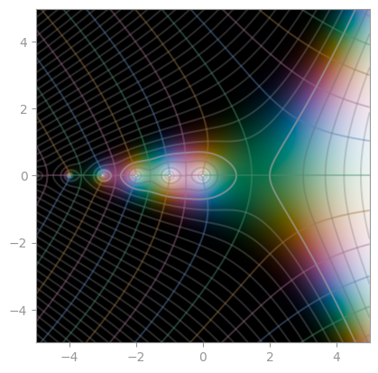
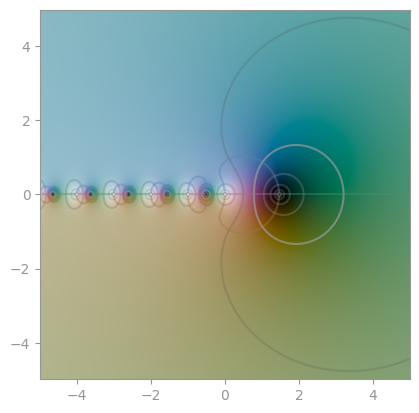
scipy.special.gamma |
scipy.special.digamma |
mpmath.zeta |
Testing
To run the cplot unit tests, check out this repository and type
pytest
License
This software is published under the GPLv3 license.
Release history Release notifications | RSS feed


Download files
Download the file for your platform. If you're not sure which to choose, learn more about installing packages.
Source Distribution
Built Distribution
Filter files by name, interpreter, ABI, and platform.
If you're not sure about the file name format, learn more about wheel file names.
Copy a direct link to the current filters
File details
Details for the file cplot-0.3.1.tar.gz.
File metadata
- Download URL: cplot-0.3.1.tar.gz
- Upload date:
- Size: 10.4 kB
- Tags: Source
- Uploaded using Trusted Publishing? No
- Uploaded via: twine/3.2.0 pkginfo/1.5.0.1 requests/2.24.0 setuptools/47.3.1 requests-toolbelt/0.9.1 tqdm/4.46.1 CPython/3.8.2
File hashes
| Algorithm | Hash digest | |
|---|---|---|
| SHA256 |
72c7a33ec4d1ebf5dd4245a75430831986d7756185fa31594923b2c0d660551c
|
|
| MD5 |
1dc297ed519397cec861d5cc43966254
|
|
| BLAKE2b-256 |
bdafdf91172aeb3e2c1c89ee419a6ba5eab6d9d8732aaca641aec9f176d2b6f0
|
File details
Details for the file cplot-0.3.1-py3-none-any.whl.
File metadata
- Download URL: cplot-0.3.1-py3-none-any.whl
- Upload date:
- Size: 20.6 kB
- Tags: Python 3
- Uploaded using Trusted Publishing? No
- Uploaded via: twine/3.2.0 pkginfo/1.5.0.1 requests/2.24.0 setuptools/47.3.1 requests-toolbelt/0.9.1 tqdm/4.46.1 CPython/3.8.2
File hashes
| Algorithm | Hash digest | |
|---|---|---|
| SHA256 |
bb11bdd8f57dab405b03ffe8fc3434447cdf8f23aa0bd66982813f9407b648d9
|
|
| MD5 |
6991496fe276053ae192ad51289da3db
|
|
| BLAKE2b-256 |
364700cd5ed5a506e9c7d9bbe7ca50b4052796794524798a0bea12114f3a48c8
|


