Density–Diversity Coresets (DDC) for dataset summarization and distributional approximation

Project description
dd-coresets
Density–Diversity Coresets (DDC): a small weighted set of real data points that approximates the empirical distribution of a large dataset.
This library exposes a simple API (in the spirit of scikit-learn) to:
- build an unsupervised density–diversity coreset (
fit_ddc_coreset); - compare against random and stratified baselines (
fit_random_coreset,fit_stratified_coreset).
The goal is pragmatic: help data scientists work with large datasets using small, distribution-preserving subsets that are easy to simulate, visualise, and explain.
Motivation
In practice, we rarely work on the full dataset for everything:
- Exploratory plots and dashboards need small, interpretable samples.
- Scenario analysis and simulations need few representative points with weights.
- Prototyping models and ideas is faster on coresets than on full data.
Common approaches:
- Random sampling: simple, but can miss important modes or tails.
- Stratified sampling: good when you already know the right strata (segments, classes, products), but needs domain knowledge and alignment with stakeholders.
- Cluster centroids (e.g. k-means): minimise reconstruction error, but centroids are not real data points and are not explicitly distributional.
DDC sits in between:
- Unsupervised, geometry-aware.
- Selects real points (medoids) that cover dense regions and diverse modes.
- Learns weights via soft assignments, approximating the empirical distribution.
Visual Example: DDC vs Random
The following example demonstrates DDC on a 2D multimodal dataset (3 Gaussian blobs + a ring structure, n=8000). We compare DDC against random sampling with the same parameters (k=80, n0=None).
Spatial Coverage
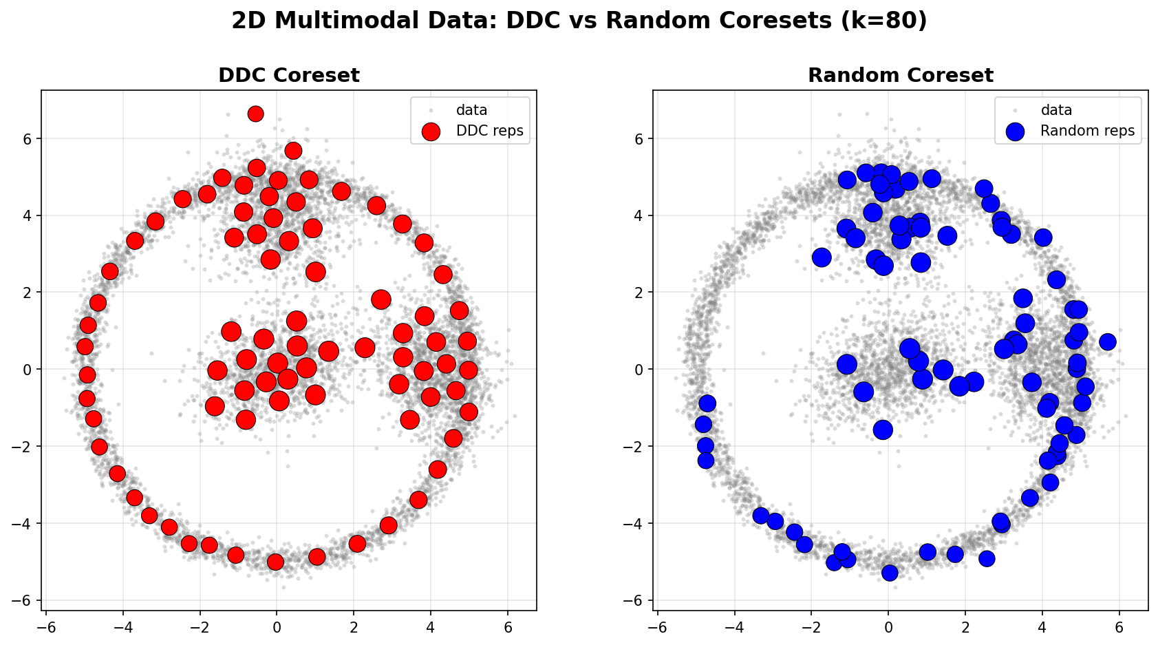
Left (DDC): Representatives are strategically placed to cover:
- All three Gaussian modes (dense regions)
- The ring structure (diverse, low-density region)
- Points are weighted by their representativeness
Right (Random): Representatives are uniformly distributed, missing the ring structure and unevenly covering the modes.
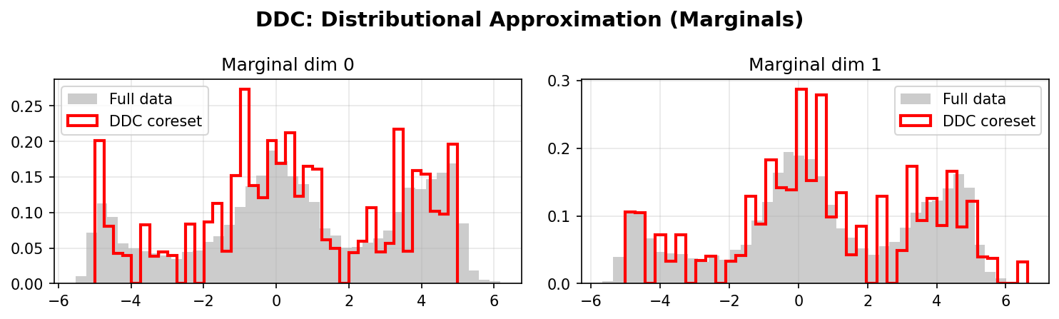
Distributional Approximation
DDC Marginals:
Random Marginals:
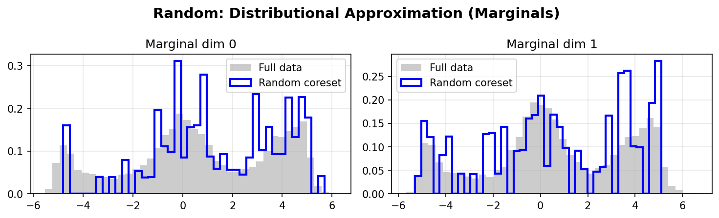
DDC better preserves the marginal distributions of the original data, especially in the tails and multimodal regions. The weighted coreset (red/blue lines) closely matches the full data distribution (gray histograms).
Quantitative Comparison
The following table compares DDC and Random coresets using standard distributional metrics:
| Method | Mean Error (L2) | Cov Error (Fro) | Corr Error (Fro) | W1 Mean | W1 Max | KS Mean | KS Max |
|---|---|---|---|---|---|---|---|
| DDC | 0.253 | 1.780 | 0.049 | 0.271 | 0.277 | 0.070 | 0.076 |
| Random | 0.797 | 2.486 | 0.080 | 0.515 | 0.806 | 0.098 | 0.138 |
Metrics explained:
- Mean Error (L2): L2 norm of the difference between full data mean and coreset weighted mean
- Cov Error (Fro): Frobenius norm of the difference between full data covariance and coreset weighted covariance
- Corr Error (Fro): Frobenius norm of the difference between correlation matrices
- W1 Mean/Max: Mean and maximum Wasserstein-1 distance across dimensions (lower is better)
- KS Mean/Max: Mean and maximum Kolmogorov-Smirnov statistic across dimensions (lower is better)
Key takeaway: DDC provides better spatial coverage and distributional fidelity than random sampling, especially when the data has multiple modes or complex geometries. Across all metrics, DDC achieves 2-3x lower error compared to random sampling.
Example: 5D Gaussian Mixture
We also compare DDC, Random, and Stratified coresets on a 5D Gaussian mixture (4 components, n=50,000). The results are visualized using UMAP 2D projection and marginal distributions.
Spatial Coverage (UMAP 2D Projection)
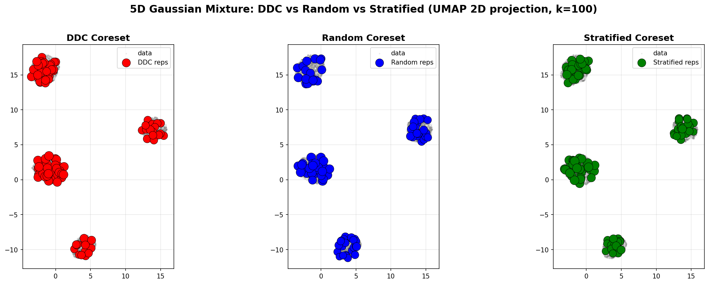
Left (DDC): Representatives are distributed across all modes, capturing the mixture structure.
Middle (Random): Representatives are uniformly scattered, missing some modes.
Right (Stratified): Representatives respect component proportions, but may miss geometric structure.
Distributional Approximation
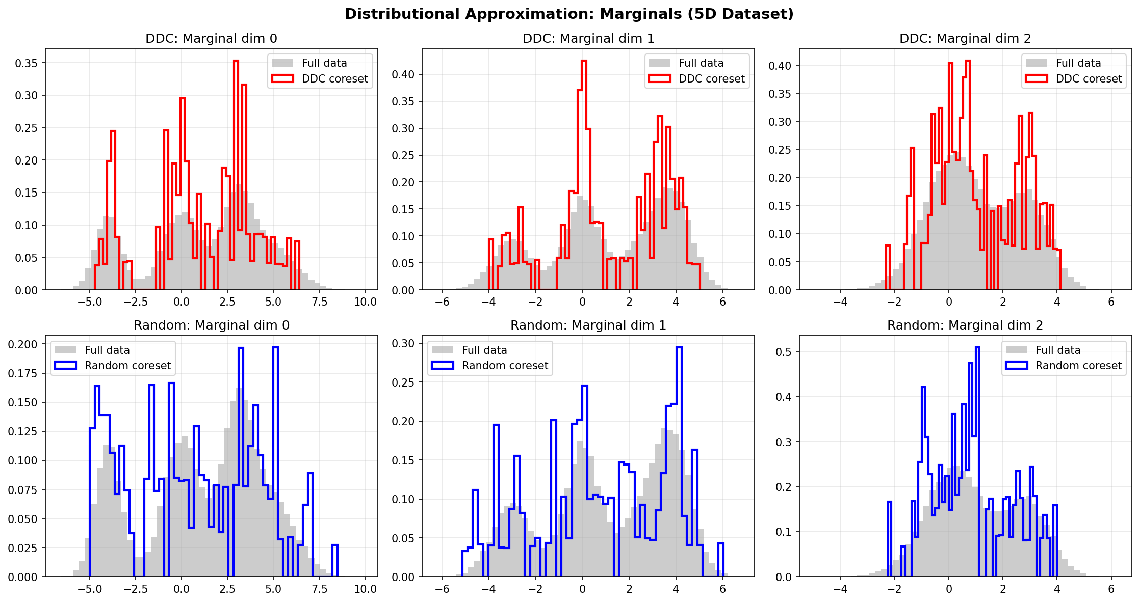
All three methods approximate the marginal distributions, with DDC and Stratified showing better fidelity to the full data distribution.
Quantitative Comparison
| Method | Mean Error (L2) | Cov Error (Fro) | Corr Error (Fro) | W1 Mean | W1 Max | KS Mean | KS Max |
|---|---|---|---|---|---|---|---|
| DDC | 0.174 | 4.197 | 0.530 | 0.251 | 0.418 | 0.073 | 0.090 |
| Random | 0.694 | 4.104 | 0.462 | 0.349 | 0.644 | 0.112 | 0.137 |
| Stratified | 0.315 | 2.708 | 0.246 | 0.213 | 0.361 | 0.063 | 0.080 |
Observations:
- DDC excels in mean approximation and Wasserstein distances (best W1 metrics).
- Stratified performs best on covariance and correlation (benefits from known component structure).
- Random shows highest errors across most metrics, confirming the value of structured sampling.
Takeaway: When component labels are available, Stratified can outperform DDC on moment-based metrics. However, DDC provides the best unsupervised performance and excels at distributional metrics (Wasserstein, KS).
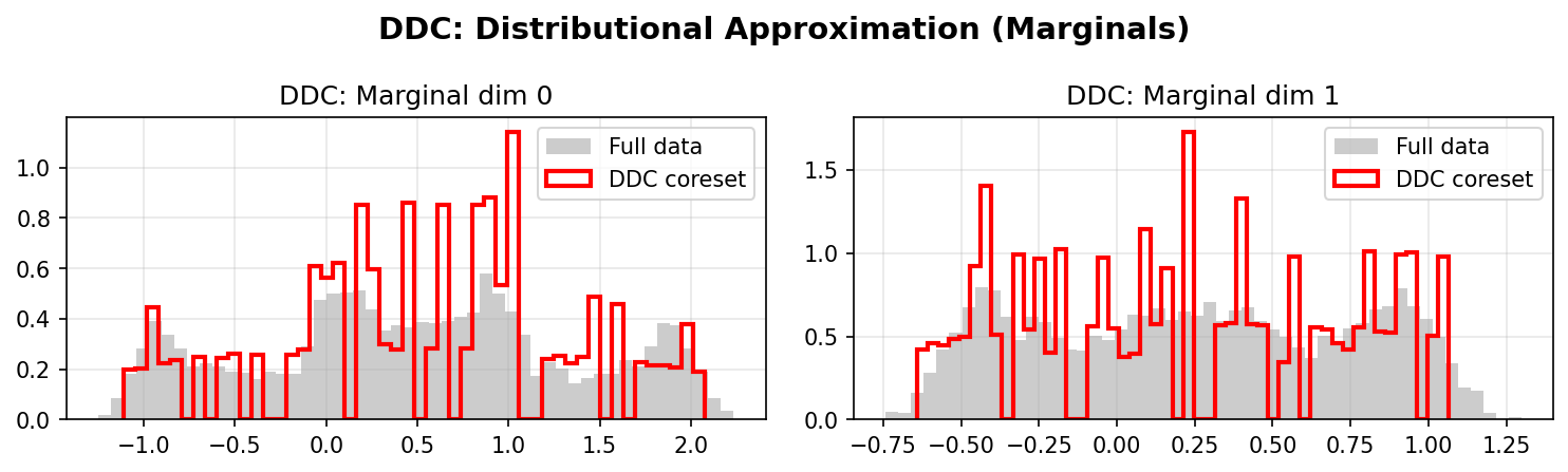
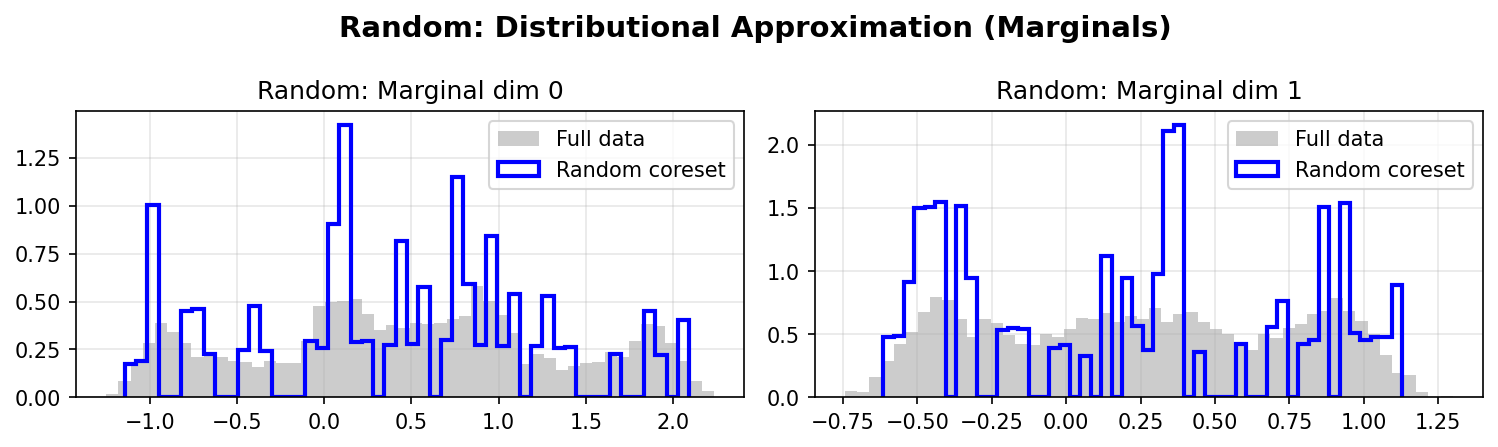
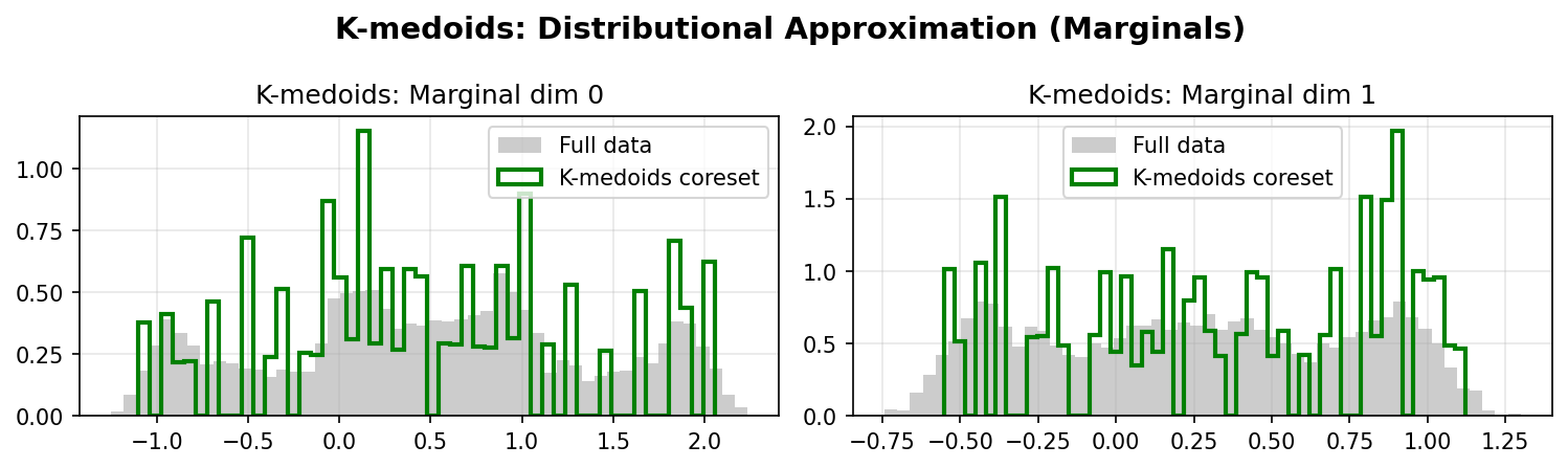
Example: Two Moons (Non-Convex Structure)
The Two Moons dataset demonstrates DDC's ability to handle non-convex structures. It consists of two interleaving half-circles (n=5000), creating a challenging geometry where random sampling and k-medoids often fail to connect both arcs.
Spatial Coverage
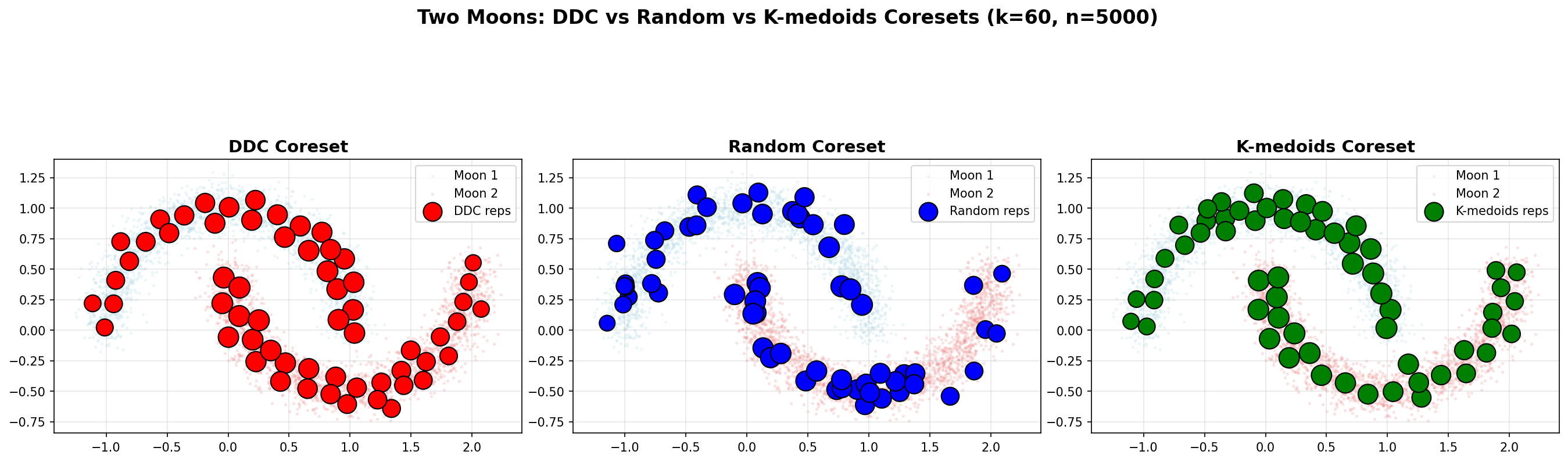
Left (DDC): Representatives are distributed along both arcs, maintaining connectivity and covering the non-convex structure.
Middle (Random): Representatives are scattered uniformly, potentially missing connections between the two moons and creating gaps.
Right (K-medoids): Representatives cluster around local centers, but may miss the connectivity between arcs due to the clustering objective.
Distributional Approximation
DDC Marginals:
Random Marginals:
K-medoids Marginals:
Quantitative Comparison
| Method | Mean Error (L2) | Cov Error (Fro) | Corr Error (Fro) | W1 Mean | W1 Max | KS Mean | KS Max |
|---|---|---|---|---|---|---|---|
| DDC | 0.069 | 0.144 | 0.006 | 0.062 | 0.094 | 0.075 | 0.081 |
| Random | 0.100 | 0.109 | 0.069 | 0.087 | 0.102 | 0.117 | 0.132 |
| K-medoids | 0.103 | 0.077 | 0.004 | 0.091 | 0.112 | 0.092 | 0.112 |
Key observations:
- DDC achieves 1.4x lower mean error than Random and 1.5x lower than K-medoids.
- DDC shows 11.5x better correlation preservation than Random and 1.5x better than K-medoids.
- DDC demonstrates superior Wasserstein and KS metrics, indicating better distributional fidelity.
- K-medoids struggles with non-convex structures, as its clustering objective focuses on minimizing within-cluster distances rather than preserving global geometry.
Takeaway: DDC excels at preserving geometric structure in non-convex datasets, outperforming both random sampling and k-medoids. This makes it particularly valuable for complex manifolds and multimodal distributions.
Installation
git clone https://github.com/crbazevedo/dd-coresets.git
cd dd-coresets

python -m venv .venv
source .venv/bin/activate  # Windows: .venv\Scripts\activate

pip install -r requirements.txt
Dependencies (minimal):
numpypandasscikit-learnmatplotlib(for examples/plots)
Quickstart
1. Fit a DDC coreset (unsupervised default)
import numpy as np
from dd_coresets.ddc import fit_ddc_coreset

# X: (n, d) preprocessed features (e.g. scaled, encoded, etc.)
X = ...  # load your data here

S, w, info = fit_ddc_coreset(
    X,
    k=200,           # number of representatives
    n0=20000,        # working sample size (None = use all)
    m_neighbors=32,  # kNN for density
    alpha=0.3,       # density–diversity trade-off
    gamma=1.0,       # kernel scale
    refine_iters=1,  # medoid refinement iters
    reweight_full=True,
    random_state=42,
)

# S: (k, d) real data points
# w: (k,) non-negative, sum to 1
# info: metadata (indices, parameters, etc.)
print(S.shape, w.shape)
print(info.method, info.k, info.n, info.n0)
You can now use (S, w) for:
- simulation / scenario analysis,
- plotting weighted histograms or KDEs,
- approximate distributional comparisons.
2. Baselines for comparison
from dd_coresets.ddc import (
    fit_random_coreset,
    fit_stratified_coreset,
    fit_kmedoids_coreset,
)

# Random coreset (no domain knowledge)
S_rnd, w_rnd, info_rnd = fit_random_coreset(
    X,
    k=200,
    n0=20000,
    gamma=1.0,
    reweight_full=True,
    random_state=0,
)

# K-medoids coreset (clustering-based)
S_kmed, w_kmed, info_kmed = fit_kmedoids_coreset(
    X,
    k=200,
    n0=20000,
    gamma=1.0,
    reweight_full=True,
    max_iters=10,
    random_state=0,
)

# Stratified coreset (when you have strata)
# strata: 1D array, same length as X, e.g. segment, class, product line
strata = ...  # e.g. y labels or business segments

S_strat, w_strat, info_strat = fit_stratified_coreset(
    X,
    strata=strata,
    k=200,
    n0=20000,
    gamma=1.0,
    reweight_full=True,
    random_state=0,
)
Use these baselines to benchmark DDC on your data (moment errors, Wasserstein distances, etc.).
API Overview
All functions assume X is a NumPy array of shape (n, d) with preprocessed numerical features (e.g. scaled, encoded, etc.).
fit_ddc_coreset
S, w, info = fit_ddc_coreset(
    X,
    k,
    n0=20000,
    m_neighbors=32,
    alpha=0.3,
    gamma=1.0,
    refine_iters=1,
    reweight_full=True,
    random_state=None,
)
-
Parameters
X:(n, d)array-like, preprocessed data.k: number of representatives.n0: working sample size. IfNoneor>= n, uses all data.m_neighbors: kNN parameter for local density.alpha: density–diversity trade-off (0 ≈ diversity,1 ≈ density).gamma: kernel scale multiplier (used in soft assignment).refine_iters: medoid refinement iterations (usually 1 is enough).reweight_full: ifTrue, reweights using the full dataset; else uses only the working sample.random_state: RNG seed.
-
Returns
S:(k, d)representatives (real data points).w:(k,)weights (w >= 0,sum(w) = 1).info:CoresetInfowith metadata (method name, n, n0, indices, params).
Recommended use:
Default choice when you do not yet know which strata or labels matter. Good for EDA, exploratory simulation, and early-stage modelling.
fit_random_coreset
S, w, info = fit_random_coreset(
    X,
    k,
    n0=20000,
    gamma=1.0,
    reweight_full=True,
    random_state=None,
)
- Samples
kpoints uniformly from a working sample (sizen0) and applies the same soft-weighting scheme as DDC.
Use case:
Baseline to compare against DDC and stratified; reflects what many teams do today (simple downsampling).
fit_stratified_coreset
S, w, info = fit_stratified_coreset(
    X,
    strata,
    k,
    n0=20000,
    gamma=1.0,
    reweight_full=True,
    random_state=None,
)
-
Parameters
X:(n, d)data.strata: 1D array of lengthnwith stratum labels (e.g. product, region, class, risk band).- Other parameters analogous to
fit_random_coreset.
-
Internally:
- Computes stratum frequencies on the working sample.
- Allocates
k_greps per stratum ∝ frequency. - Samples uniformly inside each stratum.
- Applies the same soft-weighting scheme as DDC.
Use case:
When you know the relevant strata and must preserve their proportions (regulatory reporting, risk/actuarial slices, business segments).
fit_kmedoids_coreset
S, w, info = fit_kmedoids_coreset(
    X,
    k,
    n0=20000,
    gamma=1.0,
    reweight_full=True,
    max_iters=10,
    random_state=None,
)
-
Parameters
X:(n, d)data.k: number of medoids (representatives).n0: working sample size. IfNoneor>= n, uses all data.gamma: kernel scale multiplier for soft assignments.reweight_full: ifTrue, reweights using the full dataset; else uses only the working sample.max_iters: maximum iterations for PAM-like swap optimization.random_state: RNG seed.
-
Internally:
- Uses k-means++ style initialization for medoids.
- Performs PAM-like swap optimization to minimize sum of distances to nearest medoid.
- Applies the same soft-weighting scheme as DDC.
Use case:
Clustering-based baseline that selects k real data points (medoids) minimizing within-cluster distances. Useful for comparison, but may struggle with non-convex structures.
Experiments
The repo includes three example scripts under experiments/:
-
synthetic_ddc_vs_baselines.py
5D Gaussian mixture (4 components, n=50,000):- DDC vs Random vs Stratified comparison,
- UMAP 2D visualization,
- metrics: mean/cov/corr errors, Wasserstein-1 marginals, KS.
-
multimodal_2d_ring_ddc.py
2D example (3 Gaussians + ring, n=8,000):- visual comparison DDC vs Random,
- shows how DDC covers multiple modes and a ring structure.
-
two_moons_ddc.py
2D Two Moons (non-convex structure, n=5,000):- demonstrates DDC's ability to handle non-convex geometries,
- DDC vs Random vs K-medoids comparison with quantitative metrics.
Run:
python experiments/synthetic_ddc_vs_baselines.py
python experiments/multimodal_2d_ring_ddc.py
python experiments/two_moons_ddc.py
When to use what?
-
DDC (
fit_ddc_coreset):
Default in low-knowledge regimes (no clear strata yet). Better than random sampling for a fixedk. -
Stratified (
fit_stratified_coreset):
Preferred in high-knowledge regimes (well-defined strata aligned with the task, e.g. risk bands, products), especially whenkis large enough. -
Random (
fit_random_coreset):
Baseline and sanity check; still useful when you want the simplest possible comparison. -
K-medoids (
fit_kmedoids_coreset):
Clustering-based baseline; useful for comparison but may struggle with non-convex geometries.


Download files
Download the file for your platform. If you're not sure which to choose, learn more about installing packages.
Source Distribution
Built Distribution
Filter files by name, interpreter, ABI, and platform.
If you're not sure about the file name format, learn more about wheel file names.
Copy a direct link to the current filters
File details
Details for the file dd_coresets-0.1.2.tar.gz.
File metadata
- Download URL: dd_coresets-0.1.2.tar.gz
- Upload date:
- Size: 16.1 kB
- Tags: Source
- Uploaded using Trusted Publishing? No
- Uploaded via: twine/6.2.0 CPython/3.12.9
File hashes
| Algorithm | Hash digest | |
|---|---|---|
| SHA256 |
861c95c79448af06a6e4d4d7c5eb151973e75443449241f14e9e75ad95f26347
|
|
| MD5 |
4f0bdf2db58f8cd8dfabd129d9eb9010
|
|
| BLAKE2b-256 |
2f03eb00d823aa4440527a0380fec3a1f82a0acac87f1c79e8bbd4f9c8259399
|
File details
Details for the file dd_coresets-0.1.2-py3-none-any.whl.
File metadata
- Download URL: dd_coresets-0.1.2-py3-none-any.whl
- Upload date:
- Size: 11.7 kB
- Tags: Python 3
- Uploaded using Trusted Publishing? No
- Uploaded via: twine/6.2.0 CPython/3.12.9
File hashes
| Algorithm | Hash digest | |
|---|---|---|
| SHA256 |
0fb227de9ec9af35a8a72aeb1618c651aec7725f93cc51c34ddeea38c815463c
|
|
| MD5 |
5d1122914984b7f3397c8189ec4c9a90
|
|
| BLAKE2b-256 |
d9960384dc55b18615b9c86f0434fbbd14e408f408cecbf786a6b5234919efb7
|


