
demetrapy


Run JDemetra+ TRAMO/SEATS directly from Python. demetrapy turns pandas data
into seasonally adjusted series, forecasts, diagnostics, and fitted-model
metadata without a desktop workspace or XML workflow.
Why demetrapy
- Run TRAMO/SEATS across every numeric DataFrame column with one call.
- Receive components and forecasts as date-indexed pandas DataFrames.
- Inspect diagnostics, processing messages, and fitted ARIMA models in Python.
- Assign different user-defined calendar variables to each target series.
- Reproduce reviewed workflows with typed configuration or JSON.
Install
Python 3.11+ and Java 9+ are required.
python -m pip install demetrapy
demetrapy check
To run the example notebook, install the optional Jupyter dependencies:
python -m pip install "demetrapy[notebook]"
The first adjustment downloads the pinned JDemetra+ 2.2.6 core JAR to
~/.cache/demetrapy. Set DEMETRAPY_JAR to use a local copy instead.
TRAMO/SEATS in Python
This complete example adjusts ten synthetic monthly emissions series, requests a one-year forecast, and keeps detailed model results:
from demetrapy import TramoSeatsConfig, adjust_dataframe, load_monthly_emissions

data = load_monthly_emissions()
result = adjust_dataframe(
    data,
    config=TramoSeatsConfig(
        spec="RSAfull",
        preprocessing={"automodel": {"enabled": True}},
        seats={"prediction_length": 12},
    ),
    detailed=True,
)

sa = result.sa                                   # same index/columns as data
ycal = result.ycal                               # same index/columns as data
adjusted_forecast = result.adjusted_forecast     # adjusted forecast only
all_forecasts = result.to_forecast_frame()       # every forecast component
summary = result.to_summary_frame()              # one row per input series
report = result.to_html_report("tramoseats_report.html")
power_model = result.for_series("power").arima_model

print(sa.tail())
print(ycal.tail())
print(adjusted_forecast.head())
print(summary[["series", "arima", "diagnostic_count", "forecast_periods"]])
print(power_model.notation if power_model else "Model metadata unavailable")
adjust_dataframe() infers monthly, quarterly, half-yearly, or yearly
frequency from a regular DatetimeIndex. Each column is processed
independently and every result contains six components:
| Component | Alias | Meaning |
|---|---|---|
observed |
y |
input series |
calendar_adjusted |
ycal |
calendar effects removed |
seasonally_adjusted |
sa |
seasonal effects removed |
trend |
t |
trend-cycle |
seasonal |
s |
seasonal component |
irregular |
i |
irregular component |
Select any component by compact or descriptive name, join its history and forecast, inspect processing status, or export selected components:
trend = result.component("t")
sa_forecast = result.forecast("sa")
complete_sa = result.combined("sa")
status = result.status

result.export("adjusted.csv", components=["sa"])
result.export("adjusted.xlsx", components=["sa", "ycal"])
Use to_summary_frame() to compare processing metadata across every target,
to_forecast_frame() for future values, to_combined_frame() for one
history-plus-forecast table, to_html_report() for an offline interactive
review, and for_series(name) to inspect one fitted model's diagnostics and
messages. sa and adjusted both alias the explicit seasonally_adjusted
component; ycal aliases calendar_adjusted. XLSX exports use one sheet per
selected component.
Different Calendars for Different Series
Calendar variables live in a separate DataFrame. A mapping selects which pool columns enter each target's model. Extra pool columns are allowed.
result = adjust_dataframe(
    observations,
    calendar_pool=calendar_variables,
    user_defined_calendars={
        1: [1, 3],
        "transport": ["working_days", "holiday_days", "mobility_index"],
    },
    config=config,
)
Targets and calendar variables may be selected by name or by one-based column
position. In the example, 1: [1, 3] maps the first observation column to the
first and third calendar-pool columns. Positions start at 1, not pandas' usual
zero-based position.
See the complete 10-series example with extended TRAMO/SEATS parameters: examples/13_full_config_calendar_pool.py.
Built-In Synthetic Data
All dataset loaders return fresh, deterministic pandas objects and require no
network access. load_monthly_tourism() provides hotel nights and arrivals
with multiplicative seasonality, a moving Easter effect, a level shift, and a
temporary shock. load_monthly_industrial_production() provides manufacturing,
mining, and utilities with working-day variation, a recession dip, and
additive outliers. Calendar-aware variants are available through
load_tourism_with_calendars() and
load_industrial_production_with_calendars().
More Workflows
TRAMO/SEATS is the primary workflow. The same API also supports single sequences, X13/X11, CSV automation, a command-line interface, and a Streamlit dashboard.
A sequence has no dates, so its frequency and start must be explicit:
from demetrapy import adjust

result = adjust(
    values,
    frequency="Quarterly",
    start_year=2010,
    start_period=1,
    method="tramoseats",
    spec="RSAfull",
)
For batch integration, CSV files use the same processing engine:
from demetrapy import adjust_csv

result = adjust_csv("input.csv", config="tramoseats.json", output="adjusted.csv")
X13/X11 remains available through X13Config or method="x13" when that is
the required specification.
Compare Methods and Specifications
Run any two or more labeled typed configurations against the same data:
from demetrapy import (
    TramoSeatsConfig,
    X13Config,
    compare_adjustments,
    load_monthly_retail,
    plot_comparison,
)

comparison = compare_adjustments(
    load_monthly_retail()[["sales"]],
    candidates={
        "x13-rsa4": X13Config(spec="RSA4"),
        "tramoseats-rsafull": TramoSeatsConfig(spec="RSAfull"),
    },
)

print(comparison.metrics)
print(comparison.for_series("sales").tail())
figure = plot_comparison(comparison, "sales")
figure.savefig("method_comparison.png", dpi=150)
components contains aligned results with candidate, series, and component
column levels. metrics reports pairwise RMSE, maximum absolute difference,
mean difference, and correlation for every series and component. The original
results remain available through for_candidate() for detailed inspection.
Metrics describe numerical differences; they do not select a statistically
preferred specification. plot_comparison() plots aligned candidates and a
difference panel relative to the first candidate; use component= to compare
trend, seasonal, irregular, or other components.
Command Line
demetrapy input.csv --output adjusted.csv
demetrapy init-config --method tramoseats --output config.json
demetrapy validate config.json --data input.csv
demetrapy input.csv --config config.json --output adjusted.csv --audit audit/
Dashboard
The included Streamlit dashboard runs the same X13 and TRAMO/SEATS engine as the Python API. Start with a built-in monthly, quarterly, or calendar-adjusted dataset, or upload your own files.
demetrapy-dashboard
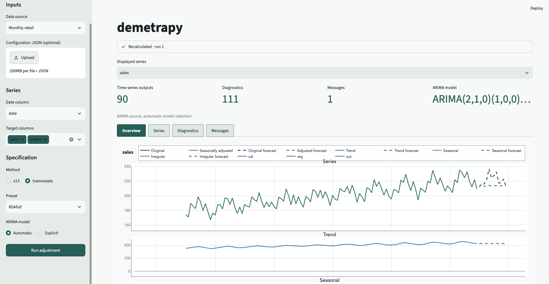
From the dashboard you can:
- adjust one or several target columns;
- preview and validate observations before processing;
- upload JSON configuration and a separate calendar-variable pool;
- map different calendar variables to each target;
- control transformation, outlier detection, and forecast horizon;
- inspect interactive components and forecasts;
- retain and compare the 10 most recent runs in the current session;
- review diagnostics, processing messages, and fitted models;
- compare X13 and TRAMO/SEATS with shared settings;
- download result tables, batch summaries, self-contained HTML reports, and a Python script that reproduces the latest successful run.
Ready-to-upload files are available in the dashboard example directory.
Documentation
- Read the documentation
- Quickstart
- Usage
- Configuration reference
- Examples
- Copy, run, inspect notebook
- Windows and offline setup
- Compatibility
demetrapy is an independent interface to JDemetra+ and is not an official
publication of the JDemetra+ project.
Alternative Solutions
If you're exploring other ways to interact with JDemetra, consider these official solutions:
- For R users: Check out rjdemetra, the official R interface for JDemetra.
- For CLI recalculations: JWSACruncher is the official command-line tool to re-calculate existing Demetra workspaces.
1 maintainer

Metadata
1 maintainer
Release files for demetrapy 0.3.10
For a detailed explanation of source distributions (sdists) and built distributions (wheels), please see the package formats documentation.
Source distribution (sdist)
| File | Size | Uploaded | |
|---|---|---|---|
| demetrapy-0.3.10.tar.gz | 86.6 kB | Details |
Built distribution (wheel)
| File | Interpreter | ABI | Platform | Reset |
|---|---|---|---|---|
| demetrapy-0.3.10-py3-none-any.whl | Python 3 | none | any | Details |
Total release size: 156.2 kB
Release files / demetrapy-0.3.10.tar.gz
| Download URL | demetrapy-0.3.10.tar.gz |
|---|---|
| Size | 86.6 kB |
| Tags | Source |
|
SHA-256 checksum How to use checksums |
cec8033c292a20bfbb35a52874652c69ccb904299fabdd77c8a8d0ab1edb086a
|
|
BLAKE2b-256 checksum How to use checksums |
46cf997bf85cd86c6412ab472de7a335798336ec1b812c934f1e00a441bceac7
|
| Upload date | |
|
Uploaded using Trusted Publishing? What is trusted publishing? |
No |
| Uploaded via |
twine/7.0.0 CPython/3.13.15
|
Release files / demetrapy-0.3.10-py3-none-any.whl
| Download URL | demetrapy-0.3.10-py3-none-any.whl |
|---|---|
| Size | 69.6 kB |
| Tags | Python 3 |
|
SHA-256 checksum How to use checksums |
d42debc51239f3ce11b6cf559986adee2502a7f9dfad408589b59972dfcb1856
|
|
BLAKE2b-256 checksum How to use checksums |
52d0cb8de746678b3849d60e6dad6b95703abf44005510d9bc30a84c3456455f
|
| Upload date | |
|
Uploaded using Trusted Publishing? What is trusted publishing? |
No |
| Uploaded via |
twine/7.0.0 CPython/3.13.15
|














