Digital logic design toolkit: simplify, minimize and transform Boolean expressions, draw KV-maps, etc.

Project description
digtick


digtick (the mnemonic for "dig tk", i.e., digital toolkit) is a command-line-tool tool for creating and solving digital logic design tasks. The primary target audiences are educators (who can use it to create and validate exam questions) and students who want to improve their skills. The toolkit allows you to specify, parse and reformat Boolean equations (e.g., output in LaTeX form for easy inclusion in documents). It can create truth tables from a given Boolean expression and rendering Karnaugh–Veitch (KV) maps with an arbitrary number of variables, both as SVG and to the command line. The output format is highly customizable to match your specific preference. It can check Boolean equations for equivalance and validate if expressions satisfy a given truth table (with counterexamples). A Quine-McCluskey implementation is used to minify expressions. digtick is able to read a subset of Logisim Evolution circuit files and is also able to simulate them natively (i.e., without relying on Logisim at all). The reason for implementing this natively within digtick is that it allows for headless interaction with circuits, e.g., to create state diagrams from circuits in an automatic fashion (see documentation of "sim-sequential" and "analyze-sequential" to make this clearer). Furthermore, digtick has the ability to randomize components within Logisim circuits (e.g., enumerate all possible gate combinations as replacement for a particular part or select a random replacement).
Boolean expression syntax
digtick accepts a pragmatic Boolean syntax that matches what students often
write on paper, while still being unambiguous and machine-parseable. Variables
follow a typical identifier pattern (e.g. A, B, clk). Constants are 0
and 1.
You can express OR as + or |, AND as * or &, and XOR as ^.
Negation can be written as !, ~, or - prefix. The parser also accepts
NAND @ and NOR % as explicit operators.
Note that neither NAND nor NOR are associative. Their precendence in parsing is as following, from strongest to weakest:
- Parenthesis: explicit
()or implicit<> - NOT
- AND
- NAND
- OR, XOR, NOR
Note that AND has higher precedence than NOR. This is so that the expression
A @ B C
is interpreted on how it is "naturally" read because of implicit AND as
A @ (B C)
instead of what would be correct if AND and NAND had same precedence:
(A @ B) C
Parentheses work as expected for grouping. Contrary to commonly used parsers,
the parser of digtick treats parenthesis as a syntactical element, which
means they are preserved in the AST. The intention is to allow for expressions
with unnecessary parenthesis to generate exam questions (students should know
that A + (B + C)) is identical to A + B + C without the parser eating away
the exam question):
$ digtick parse '(((((A | (B))))))'
(((((A + (B))))))
However, in certain cases it can be useful to have "invisible" parenthesis. For this, < and > can be used. For example:
$ digtick parse -f tex-tech 'A + !<B + C>'
\mathrm{A \vee \overline{B \vee C}}

$ digtick parse -f tex-tech 'A + !(B + C)'
\mathrm{A \vee \overline{(B \vee C)}}
Note that both expressions are correct but in the former variant the parenthesis are omitted entirely (the overline makes it clear what subexpression is inverted).
For convenience of notation, AND is implicit: adjacency separated by
whitespace counts as AND:
$ digtick parse 'A B C + A !B C + C !A'
A B C + A !B C + C !A
By default, this is also implemented this way in the output, but many commands
allow specifying a particular format, including the --no-implicit-and option:
$ digtick parse --no-implicit-and 'A B C + A !B C + C !A'
A * B * C + A * !B * C + C * !A
There are multiple output options, e.g. a Unicode renderer:
$ digtick parse --expr-format pretty-text 'A B C + A !B C + C !A'
A B C ∨ A B̅ C ∨ C A̅
Operator precedence within Python
Note that, when importing digtick and using it to perform changes under the
hood, you can also naturally use the overloaded operators. They also automatically convert
strings and integers to variables and constants. Example:
from digtick.ExpressionParser import Variable
(A, B, C) = (Variable("A"), Variable("B"), Variable("C"))
print(~((A | B) & C))
>>> [![[A + B] * C]]
Note that also the @ and % operators are overloaded to provide NAND and
NOR, but with the caveat that the operator precedence within Python is
different than our parsing precedence!
from digtick.ExpressionParser import Variable
(A, B, C) = (Variable("A"), Variable("B"), Variable("C"))
print(A @ B & C == (A @ B) & C)
>>> True
Truth table format
There is a human-readable truth table format which uses Unicode characters for pretty viewing in a terminal and the machine-readable format which is whitespace-separated. The latter is the default output variant one of two forms which can be used as input:
$ digtick make-table 'A B C + A !B C + C !A'
A	B	C   >Y
0	0	0	0
0	0	1	1
0	1	0	0
0	1	1	1
1	0	0	0
1	0	1	1
1	1	0	0
1	1	1	1

$ digtick make-table --tbl-format pretty 'A B C + A !B C + C !A'
┌───┬───┬───┬───┐
│ A │ B │ C │ Y │
├───┼───┼───┼───┤
│ 0 │ 0 │ 0 │ 0 │
│ 0 │ 0 │ 1 │ 1 │
│ 0 │ 1 │ 0 │ 0 │
│ 0 │ 1 │ 1 │ 1 │
│ 1 │ 0 │ 0 │ 0 │
│ 1 │ 0 │ 1 │ 1 │
│ 1 │ 1 │ 0 │ 0 │
│ 1 │ 1 │ 1 │ 1 │
└───┴───┴───┴───┘
By default, the output is named Y. Output signals are denoted by the >
prefix in the heading row. There can be multiple output signals in a single table.
Note that commands which accept truth table inputs can all have the filename omitted and will then read from stdin. This allows for easy piping of commands:
$ digtick make-table 'A B C + A !B C + C !A' | digtick synth
CDNF: !A !B C + !A B C + A !B C + A B C
CCNF: (A + B + C) (A + !B + C) (!A + B + C) (!A + !B + C)
DNF : C
CNF : (C)
There is a second format which is also automatically accepted, called the "compact" format. The compact format is useful when you want to modify whole tables in a single command line because it is, as the name indicates, a very compact representation of a truth table:
$ digtick make-table --tbl-format compact 'A B C + A !B C + C !A'
:A,B,C:Y:4444
digtick distinguishes when reading table input by the first character of the
first line -- in compact format, this is always a colon :. Compact format
then lists the input variable names, output variable names and then the
bit-packed data (0 = Low, 1 = High, 2 = Don't Care, 3 = Undefined). Note the
seamless conversion:
$ echo :A,B,C:Y:4444 | digtick print-table
A	B	C	>Y
0	0	0	0
0	0	1	1
0	1	0	0
0	1	1	1
1	0	0	0
1	0	1	1
1	1	0	0
1	1	1	1
Timing diagram format
For timing diagrams (described below in more detail), the general format is this:
# Comment, this will be ignored
A  = 01010101010101010
!B = 10101010101010101
This shows two signals, A and !B. Characters that can be used are:
0/1: LOW or HIGH:: both LOW and HIGH (invalid/ambiguous state)!: LOW -> HIGH and HIGH -> LOW transition simultaneous (only valid within:blocks to indicate a signal may change)Z: High impedance (middle line)|: Marker line at that exact point. May also be a labeled marker by using|'text'._: Empty clock cycle
Whitespace is ignored.
"parse": parse and reformat Boolean expressions
parse parses an equation and outputs it in a different format, such as LaTeX.
It takes care that in overline-style negation of literals the overline does
not automatically carry over to the next character (this is an annoying LaTeX
default, unfortunately, and results in a non-equivalent equation):
$ digtick parse --expr-format tex-tech '!A !B'
\overline{\textnormal{A}} \ \overline{\textnormal{B}}
$ digtick parse --expr-format tex-tech '!(A B)'
\overline{(\textnormal{A} \ \textnormal{B})}
Note that also the mathematical variant of symbols can be used:
$ digtick parse --expr-format tex-math '!(A B)'
\neg \textnormal{A} \ \neg \textnormal{B}
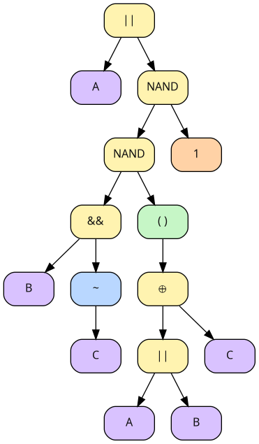
When you are interested in the internal parse tree of an expression, you can emit the expression as Graphviz-compatible format and have it rendererd by dot into a graph:
$ digtick parse --expr-format dot 'A + B -C @ (A + B ^ C) @ 1' | dot -Tpng -oast.png
Which will produce the following ast.png file:
digtick is also able to produce Typst-compatible output, but note that it needs the following macros to be defined in your document:
#let bnand = box(width: 1em, height: 0.6em)[#place(center, dy: -0.1em)[#sym.and] #place(center, dy: -0.1em)[#text(size: 0.85em)[#sym.tilde]]]
#let bnor = box(width: 1em, height: 0.6em)[#place(center, dy: -0.1em)[#sym.or] #place(center, dy: -0.1em)[#text(size: 0.85em)[#sym.tilde]]]
#let bnot(body) = $overline(#v(1em)#h(0em) body)$
"make-table": generate a truth table from an expression
make-table evaluates a Boolean expression over all input combinations and
prints a truth table. An optional second expression can be used to mark “don't
care” output positions (*). Wherever the “don't care” expression evaluates to
1, the output is printed as * instead of 0 or 1.
$ digtick make-table 'A + B !C' 'A !B'
A	B	C   >Y
0	0	0	0
0	0	1	0
0	1	0	1
0	1	1	0
1	0	0	*
1	0	1	*
1	1	0	1
1	1	1	1
"print-table": read and print a table file
print-table reads a TSV truth table and prints it back in either plain TSV
form or a formatted view. If your table doesn't define every input combination,
you can decide how missing patterns should be treated. In the default strict
mode, missing patterns are considered an error; in the relaxed modes, missing
patterns are filled as 0, 1, or *.
$ digtick make-table 'A + B !C' 'A !B' | \
  head -n 4 | \
  digtick print-table -f pretty --unused-value-is '*'
┌───┬───┬───┬───┐
│ A │ B │ C │ Y │
├───┼───┼───┼───┤
│ 0 │ 0 │ 0 │ 0 │
│ 0 │ 0 │ 1 │ 0 │
│ 0 │ 1 │ 0 │ 1 │
│ 0 │ 1 │ 1 │ * │
│ 1 │ 0 │ 0 │ * │
│ 1 │ 0 │ 1 │ * │
│ 1 │ 1 │ 0 │ * │
│ 1 │ 1 │ 1 │ * │
└───┴───┴───┴───┘
"kv": render a Karnaugh–Veitch map from a table
kv takes a truth table and lays it out as a KV map. There are multiple ways
to create a KV map which are all. As an educator, I usually have the policy
that my students need not adhere to the format taught in my lectures, but may
choose a different format as long as it produces correct output. This puts the
burden of verification on me, which is cumbersome. For this purpose, this
rendering command accepts a number of different parameters that influence the
way the KV diagram is printed.
$ digtick make-table 'A B !C + B D + !C A' 'B !A D + A B C D' >examples/table1.txt
$ digtick kv examples/table1.txt
┌─────┬─────┬─────┬─────┬─────┐
│     │ A̅ B̅ │ A B̅ │ A B │ A̅ B │
├─────┼─────┼─────┼─────┼─────┤
│ C̅ D̅ │  0  │  1  │  1  │  0  │
├─────┼─────┼─────┼─────┼─────┤
│ C D̅ │  0  │  0  │  0  │  0  │
├─────┼─────┼─────┼─────┼─────┤
│ C D │  0  │  0  │  *  │  *  │
├─────┼─────┼─────┼─────┼─────┤
│ C̅ D │  0  │  1  │  1  │  *  │
└─────┴─────┴─────┴─────┴─────┘

$ digtick kv examples/table1.txt -d DCBA --x-offset 1 --y-invert
┌─────┬─────┬─────┬─────┬─────┐
│     │ C̅ D │ C D │ C D̅ │ C̅ D̅ │
├─────┼─────┼─────┼─────┼─────┤
│ A̅ B̅ │  0  │  0  │  0  │  0  │
├─────┼─────┼─────┼─────┼─────┤
│ A B̅ │  1  │  0  │  0  │  1  │
├─────┼─────┼─────┼─────┼─────┤
│ A B │  1  │  *  │  0  │  1  │
├─────┼─────┼─────┼─────┼─────┤
│ A̅ B │  *  │  *  │  0  │  0  │
└─────┴─────┴─────┴─────┴─────┘
This makes it much easier to verify solutions for their correctness, regardless of which format the student chose.
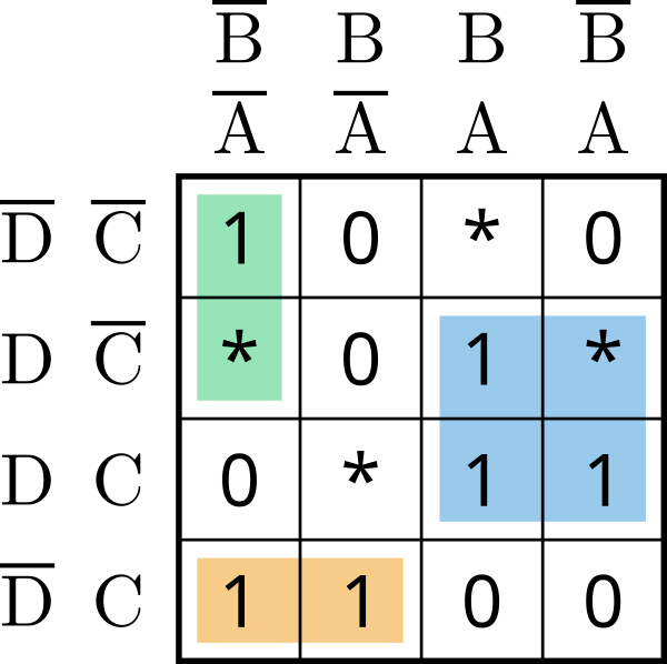
You may also render SVGs from a KV diagram, which will also display the solution implicants for both DNF and CNF using SVG layers:
$ digtick kv --output-filename docs/kv.svg examples/table2.txt
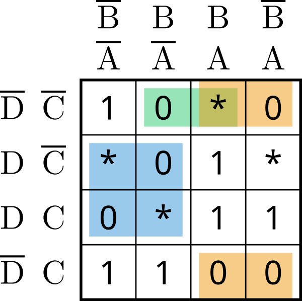
Via layers, you can also switch to CNF view:
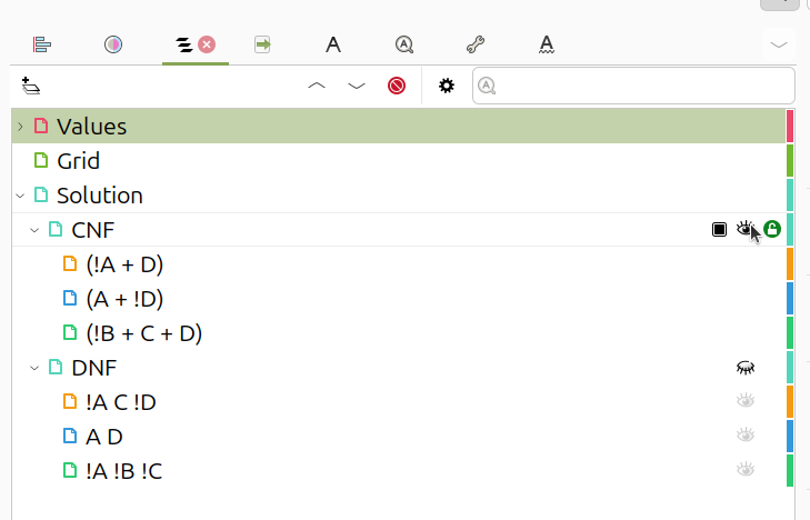
The selection, here shown in Inkscape, allows also for selection based on single min/maxterms:
"synthesize": minimize/synthesize expressions from a truth table
synthesize reads a truth table and prints canonical forms (CDNF/CCNF) as well
as minimized forms (DNF/CNF) produced via Quine-McCluskey.
$ digtick synth exam1.txt
CDNF: A !B !C !D + A !B !C D + A B !C !D + A B !C D
CCNF: (A + B + C + D) (A + B + C + !D) (A + B + !C + D) (A + B + !C + !D) (A + !B + C + D) (A + !B + !C + D) (!A + B + !C + D) (!A + B + !C + !D) (!A + !B + !C + D)
DNF : A !C + B D
CNF : (!C) (A)
The Quine-McCluskey implementation uses the classical approach (creating the Prime Implicant chart, then run Petrick's Method to determine Implicant coverage). It tries to minimize the number of minterms/maxterms and only as a secondary objective tries to minimize the number of literals. I am not fully certain but am quite convinced that minimizing number of implicants also implicitly minimizes number of literals used. In any case I was unable to find a counterexample (if you have one, absolutely reach out please -- also if you do find proof that my reasoning is correct).
The implementation is not the fastest because of the algorithm used and will, for complicated charts, take some time:
$ time echo ":A,B,C,D,E,F:Y:1064158620815865a044911508155600" | digtick synth -c dnf
CDNF: A B C !D E !F + A B C !D !E F + A B C !D !E !F + A B !C D E F + A B !C D E !F + A B !C D !E F + A !B C D E F + A !B C D E !F + A !B C D !E F + A !B C !D E F + A !B C !D !E F + A !B !C D E !F + A !B !C D !E !F + !A B C D E F + !A B C D E !F + !A B C D !E !F + !A B C !D !E F + !A B C !D !E !F + !A B !C D E F + !A !B C D E !F + !A !B C !D E F + !A !B C !D E !F + !A !B C !D !E F + !A !B !C D E !F + !A !B !C D !E !F + !A !B !C !D !E F
DNF : B C !D F + B !D !E F + !A B !C !F + !A !B !C D + A B !C !E + A D E !F + A !B !C F + !A !B C !D !E + A !B !D !E !F + !A !B C !D !F

real	0m0,536s
user	0m0,518s
sys	0m0,018s
One advantage of this approach is that we get similar cost terms after the fact. Again, this is important for exam work (your exam question may have more than one valid, perfectly correct, answer):
$ echo ":A,B,C,D:Y:4285568" | digtick synth --show-all-solutions
CDNF: A B !C !D + A !B C D + A !B C !D + A !B !C D + A !B !C !D + !A !B C !D
DNF 1/2: !A B + !A D + !C D
DNF 2/2: !A B + !A C + !C D

CCNF: (!A + !B + !C + !D) (A + !B + !C + !D) (A + !B + C + D) (A + B + !C + !D) (A + B + C + !D) (A + B + C + D)
CNF 1/2: (B + C) (!A + D) (!A + !C)
CNF 2/2: (B + D) (!A + D) (!A + !C)
Note that there are two solutions identical in number of minterms/maxterms for both DNF and CNF, both with the identical number of literals and negations (although negations are ignored in judging cost of expressions). This allows you to randomly generate tables to either provoke or avoid such a scenario.
"equal": check whether two expressions are equivalent
equal compares two Boolean expressions by evaluating them over all possible
input assignments of the involved variables. If they are equivalent, it reports
success. If they differ, it prints a counterexample assignment.
$ digtick eq 'A @ B @ C' 'A @ (B @ C)'
Not equal: {'A': 0, 'B': 0, 'C': 1} gives 0 on LHS but 1 on RHS

$ digtick eq 'A B C + C !D B + B C' 'B C'
Expressions equal.
Note that digtick also supports checking a whole file for equivalence in the parse command. For example, say you have generated an exam and are preparing the reference solution, in which you are performing tiny simplification steps each line:
$ cat examples/equations.txt
A B C + B C (A + D) + B A !D + F (E + !F)
A B C + B C A + B C D + B A !D + F (E + !F)
A B C + B C A + B C D + B A !D + F E + F !F
A B C + B C A + B C D + B A !D
B C A + B C D + B A !D
B (C A + C D + A !D)
B (C D + A !D)
Did you spot my error? A simple omission that changes the whole formula:
$ digtick parse --read-as-filename --validate-equivalence examples/equations.txt
A B C + B C (A + D) + B A !D + F (E + !F)
A B C + B C A + B C D + B A !D + F (E + !F)
A B C + B C A + B C D + B A !D + F E + F !F
A B C + B C A + B C D + B A !D
Warning: expression "A * B * C + B * C * A + B * C * D + B * A * !D + F * E + F * !F" on line 3 is not equivalent to expression "A * B * C + B * C * A + B * C * D + B * A * !D" on line 4.
B C A + B C D + B A !D
B (C A + C D + A !D)
B (C D + A !D)
There were validation errors, some of the equations are not equivalent to each other.
You can also render all these expressions to TeX syntax; this is especially
annoying to write manually because TeX by default merges adjacent \overline{}
statements; i.e., when you have the expression A B and write \overline{A} \overline{B}, TeX will create only a single overline which makes a completely
different expression: ~(AB). Since I've been bitten by this too often, now I
only generate TeX. I'm sure you'll agree that this output is a write-only
format not intended for human consumption:
$ digtick parse -f tex-tech 'A C !(B + !(D + !E)) + E + A !B !C D !E !F G'
\mathrm{A C \overline{(B \vee \overline{(D \vee \overline{E})})} \vee E \vee A \overline{B}\,\overline{C} D \overline{E}\,\overline{F} G}
Note that digtick inserts half spaces \, where two overlines would be merged,
but not where they are not needed. Obviously, a whole file can also be
converted to TeX (and also not only is overline syntax usable but also the
mathematical notation of Boolean expressions):
$ digtick parse -f tex-math --read-as-filename examples/equations.txt
\mathrm{A B C \vee B C (A \vee D) \vee B A \neg D \vee F (E \vee \neg F)}
\mathrm{A B C \vee B C A \vee B C D \vee B A \neg D \vee F (E \vee \neg F)}
\mathrm{A B C \vee B C A \vee B C D \vee B A \neg D \vee F E \vee F \neg F}
\mathrm{A B C \vee B C A \vee B C D \vee B A \neg D}
\mathrm{B C A \vee B C D \vee B A \neg D}
\mathrm{B (C A \vee C D \vee A \neg D)}
\mathrm{B (C D \vee A \neg D)}
"satisfied": Validate a solution against a truth table
satisfied takes a truth table as input as well as a Boolean expression and
verifies that the expression indeed fulfills the truth table. It prints the
locations where it is not fulfilled, again in table format:
$ digtick satisfied -f pretty examples/table1.txt 'A !(A !B C)'
┌───┬───┬───┬───┬───┬──────┬─────┐
│ A │ B │ C │ D │ Y │ Eval │ Sat │
├───┼───┼───┼───┼───┼──────┼─────┤
│ 0 │ 0 │ 0 │ 0 │ 0 │ 0    │ 1   │
│ 0 │ 0 │ 0 │ 1 │ 0 │ 0    │ 1   │
│ 0 │ 0 │ 1 │ 0 │ 0 │ 0    │ 1   │
│ 0 │ 0 │ 1 │ 1 │ 0 │ 0    │ 1   │
│ 0 │ 1 │ 0 │ 0 │ 0 │ 0    │ 1   │
│ 0 │ 1 │ 0 │ 1 │ * │ 0    │ 1   │
│ 0 │ 1 │ 1 │ 0 │ 0 │ 0    │ 1   │
│ 0 │ 1 │ 1 │ 1 │ * │ 0    │ 1   │
│ 1 │ 0 │ 0 │ 0 │ 1 │ 1    │ 1   │
│ 1 │ 0 │ 0 │ 1 │ 1 │ 1    │ 1   │
│ 1 │ 0 │ 1 │ 0 │ 0 │ 0    │ 1   │
│ 1 │ 0 │ 1 │ 1 │ 0 │ 0    │ 1   │
│ 1 │ 1 │ 0 │ 0 │ 1 │ 1    │ 1   │
│ 1 │ 1 │ 0 │ 1 │ 1 │ 1    │ 1   │
│ 1 │ 1 │ 1 │ 0 │ 0 │ 1    │ 0   │
│ 1 │ 1 │ 1 │ 1 │ * │ 1    │ 1   │
└───┴───┴───┴───┴───┴──────┴─────┘
Warning: the given expression does NOT satisfy the truth table


$ digtick satisfied -f pretty examples/table1.txt 'A !(A !B C) !(A B C !D)'
┌───┬───┬───┬───┬───┬──────┬─────┐
│ A │ B │ C │ D │ Y │ Eval │ Sat │
├───┼───┼───┼───┼───┼──────┼─────┤
│ 0 │ 0 │ 0 │ 0 │ 0 │ 0    │ 1   │
│ 0 │ 0 │ 0 │ 1 │ 0 │ 0    │ 1   │
│ 0 │ 0 │ 1 │ 0 │ 0 │ 0    │ 1   │
│ 0 │ 0 │ 1 │ 1 │ 0 │ 0    │ 1   │
│ 0 │ 1 │ 0 │ 0 │ 0 │ 0    │ 1   │
│ 0 │ 1 │ 0 │ 1 │ * │ 0    │ 1   │
│ 0 │ 1 │ 1 │ 0 │ 0 │ 0    │ 1   │
│ 0 │ 1 │ 1 │ 1 │ * │ 0    │ 1   │
│ 1 │ 0 │ 0 │ 0 │ 1 │ 1    │ 1   │
│ 1 │ 0 │ 0 │ 1 │ 1 │ 1    │ 1   │
│ 1 │ 0 │ 1 │ 0 │ 0 │ 0    │ 1   │
│ 1 │ 0 │ 1 │ 1 │ 0 │ 0    │ 1   │
│ 1 │ 1 │ 0 │ 0 │ 1 │ 1    │ 1   │
│ 1 │ 1 │ 0 │ 1 │ 1 │ 1    │ 1   │
│ 1 │ 1 │ 1 │ 0 │ 0 │ 0    │ 1   │
│ 1 │ 1 │ 1 │ 1 │ * │ 1    │ 1   │
└───┴───┴───┴───┴───┴──────┴─────┘
The given expression satisfies the truth table.
"random-expr": generate a random Boolean expression
random-expr generates a random expression over a specified number of
variables that has a certain "complexity" according to some metric (currently,
number of generated minterms/maxterms). It automatically simplifies the
randomized equations and checks that the minimized variant is not below another
complexity metric (so that tautologies are not created unless the user
specifically specifies that simple results are permissible via
--allow-trivial):
$ digtick random-expr 4 60
Expression: !((!B !C D A + A C)) (!C) !B !C (!D + !C) + (!C + D) B C D A + !B !A
Simplified: !B !C !D + !A !B + A B C D
"random-table": generate a random truth table
random-table creates a truth table for a specified number of variables,
randomly choosing output values according to configured probabilities. By
default the output distribution is 40% zeros, 40% ones, and the remainder
don't-cares. You can adjust the zero/one percentages; whatever remains after
those is implicitly treated as *.
$ digtick random-table -0 30 -1 50 3
A	B	C   >Y
0	0	0	0
0	0	1	1
0	1	0	*
0	1	1	*
1	0	0	1
1	0	1	1
1	1	0	1
1	1	1	0
"transform": Transform a Boolean expression
transform allows you to input a Boolean expression and have it converted into
NAND or NOR logic, i.e., replacing all gates exclusively by NAND or NOR.
Examples:
$ digtick transform -t nand 'A ^ B'
((A @ 1) @ B) @ (A @ (B @ 1))

$ digtick transform -t nor 'A ^ !B'
((A % ((B % 0) % 0)) % ((A % 0) % (B % 0)) % 0)
Note that, as stated above, @ is shortcut notation for NAND while % stands
for NOR.
Other notable transformation are the "simplify" transformation which attempts to algorithmically simplify expressions. Note that this is quite basic functionality:
$ digtick transform -t simplify 'A + A B A + (C @ 1 @ 1)'
A + C + A B
As you can see, the redundant term "AB" is not removed in the above example, although it is clearly covered by "A".
Expressions can also be rearranged/shuffled. This is useful to prepare randomized student questions which are all identical (but different). Note that there is an iteration paraemter that you can use as well to generate multiple variants:
$ digtick random-expr 4 5
Expression: (!D C !B !C !D A + !A !D !C) !D !B + !C A B D
Simplified: A B !C D + !A !B !C !D

$ digtick transform -I 5 -t shuffle '(!D C !B !C !D A + !A !D !C) !D !B + !C A B D'
B !C D A + !B (!D !A !C + !D !B !D !C C A) !D
(!A !D !C + C !B !D !D !C A) !D !B + !C B A D
!B (!C !D !A + !D C A !B !C !D) !D + !C B D A
!D !B (!C !A !D + !C !B A C !D !D) + A D B !C
(!D !D A !B C !C + !C !D !A) !B !D + D !C B A
Lastly, there is a transformation that exclusively sorts literals and subexpressions to create a standard form:
$ digtick transform -t sort '(!D !D A !B C !C + !C !D !A) !B !D + D !C B A'
!B !D (!A !C !D + A !B C !C !D !D) + A B !C D
"dtd-create": Create a digital timing diagram
dtd-create generates timing-diagram source text (a compact, line-based
format) for common sequential devices typically used in exam exercises: SR-NAND
flipflops, D-flipflops, JK- or JK-MS-flipflops. It produces randomized inputs
(reproducible via a seed), simulates the device, and prints input/output
waveforms.
To do this, you can simply invoke the command and it will generate a random timing diagram (by default of a SR-NAND-FF):
$ digtick dtd-create
# Random seed: 8910607998
!S = 0|'S'0|'R'11|0|'🗲'111|00|'R'111111|'S'0000|00|'S'00000111|'R'11
!R = 0    1    00 0    111 00    000001    1111 00    11111111    01
Q  = 1    1    00 1    000 11    000000    1111 11    11111111    00
!Q = 1    0    11 1    111 11    111111    0000 11    00000000    11
As you can see, it created a diagram along with notational markers that show when the flipflop was set, when it was reset and where an illegal state transition occurred. Note that for the SR-NAND-FF it is not illegal for both inputs to become active (i.e., LOW) at the same time, this is well-defined behavior. Undefined behavior occurs only when out of this state there is a simultaneous transition into the "keep" state (both inputs inactive, i.e., HIGH).
You can also predefine certain values if you wish, but the specified signal length must match exactly with the length of the graph you choose:
$ digtick dtd-create -d d-ff C=00011100011100011100011100011100
# Random seed: 1015274594
C  = 000|111000|111000|111000|111000|11100
D  = 000 000001 111111 011111 000000 00000
Q  = 000 000000 111111 111111 111111 00000
!Q = 111 111111 000000 000000 000000 11111
"dtd-render": render timing diagram data to SVG
dtd-render reads timing-diagram source text (from a file or stdin) and
renders it as an SVG. As an example, consider the example shown before in
dtd-create. Let us reproduce it from its pseudo-random seed and render it:
$ digtick dtd-create -s 8910607998 | digtick dtd-render -o /tmp/timing_diagram.svg
Will create the file /tmp/timing_diagram.svg which you can see here (note
that here, a PNG-conversion is shown which is why it looks fuzzy/washed out --
the original is crystal clear):
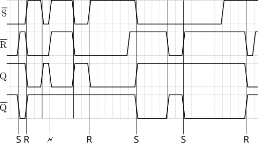
Note that the two-step process makes it exceptionally easy to create random diagrams until you find one that you like, use this as the reference solution for an exam, edit the test file and clear out the signals you want students to fill in, then render that again.
Also note that the created SVG supports layers so it is easy to retroactively disable, for example, labels or tick markers.
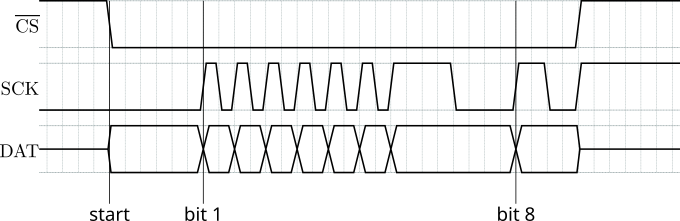
Another example is this timing diagram, showing tri-state states:
!CS = 1111|'start'000000        00000000000000000000        00001111111
SCK = 0000        000000|'bit 1'10101010101011110000|'bit 8'11001111111
DAT = ZZZZ        ::::::        !:!:!:!:!:!:!:::::::        !:::ZZZZZZZ
Which renders as:
"sim-combinatorial": Simulate a stateless Logisim Evolution circuit
With sim-combinatorial you can simulate simple combinatorial circuits that
are given as Logisim Evolution files. The file is read, all sources are
treated as inputs and all sinks are treated as outputs. The result is a truth
table:
$ digtick sim-combinatorial -f pretty examples/full-adder.circ
┌───┬───┬─────┬──────┬───┐
│ A │ B │ Cin │ Cout │ S │
├───┼───┼─────┼──────┼───┤
│ 0 │ 0 │ 0   │ 0    │ 0 │
│ 0 │ 0 │ 1   │ 0    │ 1 │
│ 0 │ 1 │ 0   │ 0    │ 1 │
│ 0 │ 1 │ 1   │ 1    │ 0 │
│ 1 │ 0 │ 0   │ 0    │ 1 │
│ 1 │ 0 │ 1   │ 1    │ 0 │
│ 1 │ 1 │ 0   │ 1    │ 0 │
│ 1 │ 1 │ 1   │ 1    │ 1 │
└───┴───┴─────┴──────┴───┘
"sim-sequential": Simulate a stateful Logisim Evolution circuit
The sim-sequential command allows you to examine a stateful sequential
circuit regarding its behavior after a clock edge. It iterates through all
possible state combinations as inputs, simulates a clock cycle and reads the
state values back out. The output is a truth table with n input values and n
output values, resembling the state of the storage elements before and after
the clock edge. For example, consider this circuit:
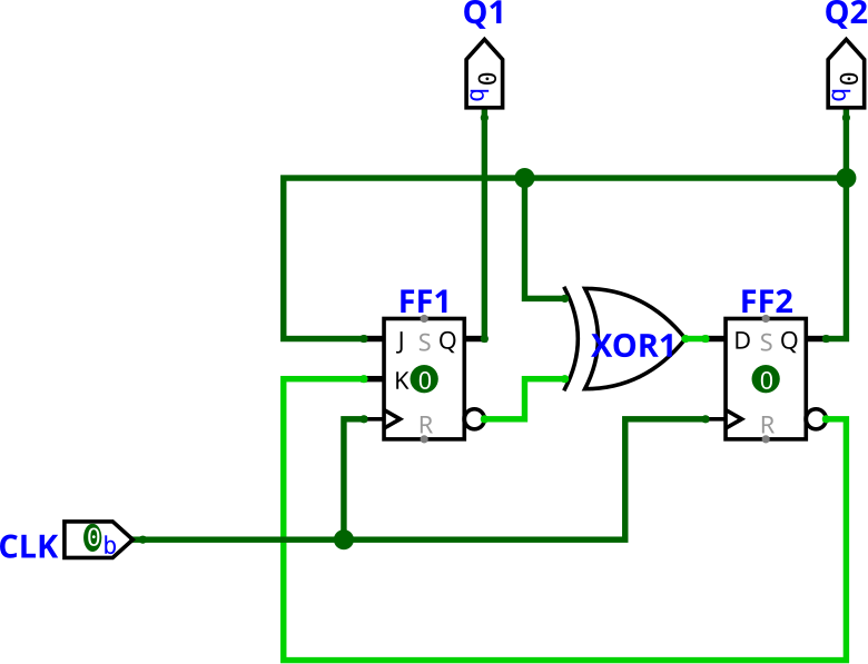
A typical exam question could be to assume reset and show the outputs in the next 2 clock cycles. However, as an educator you need to deal with answers which are off by one bit, which can throw everything off. When you design a circuit that has a fix point, this could make the exam question much easier for certain combinations -- how do you fairly judge that answer? That problem goes away entirely when the circuit is designed so that any input combination is approximately the same difficulty as each other one, ideally forming a completely cyclic graph. In Logisim Evolution, this is a manual task and fairly labor intensive. This is why you can simply use digtick for that purpose:
$ digtick sim-sequential -s FF1,FF2 -f pretty examples/simple-ff.circ
┌─────┬─────┬──────┬──────┐
│ FF1 │ FF2 │ FF1' │ FF2' │
├─────┼─────┼──────┼──────┤
│ 0   │ 0   │ 0    │ 1    │
│ 0   │ 1   │ 1    │ 0    │
│ 1   │ 0   │ 0    │ 0    │
│ 1   │ 1   │ 1    │ 1    │
└─────┴─────┴──────┴──────┘
This allows you to create a table in which you can look up for each state what the successor state is. While this representation may be useful for certain things (like correcting an exam), it is not as easy to see where fixpoints are, especially when circuits are more complicated. For this reason, the "analyze-sequential" tool is available.
"analyze-sequential": Analyze state transitions in sequential circuits
After the sim-sequential command has generated a state truth table,
analyze-sequential then can take that table as input and displays the
topology of the state graph, i.e., the transitions between states:
$ digtick sim-sequential -s FF1,FF2 examples/simple-ff.circ >/tmp/states.txt
$ digtick analyze-sequential /tmp/states.txt
State transitions: FF1, FF2 → FF1', FF2'
   Cycle ID=0 length 3: 0 → 1 → 2 → 0
   Cycle ID=3 length 1: 3 → 3
State graph has 2 cycles and 0 tails. Shortest cycle length: 1
State graphs must always be cyclic (they are finite, after all) but circuits with short cycles are unsuitable as exam questions (a student might miscalculate, end up in a cycle and then get "stuck").
While this circuit was a fairly easy example, let's examine at a more complex circuit, where transitions are not as straightforward anymore:
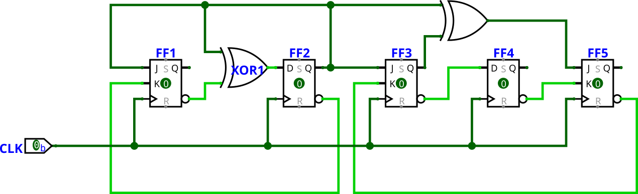
It is not straightforward to see how this circuit behaves and even when analyzing it textually, this is only somewhat useful:
$ digtick sim-sequential -s FF1,FF2,FF3,FF4,FF5 examples/complex-ff.circ >/tmp/states.txt
$ digtick analyze-sequential /tmp/states.txt
State transitions: FF1, FF2, FF3, FF4, FF5 → FF1', FF2', FF3', FF4', FF5'
   Cycle ID=2 length 6: 2 → 10 → 23 → 5 → 12 → 16 → 2
   Cycle ID=24 length 4: 24 → 31 → 29 → 28 → 24
   Tail length 1: 0 → [ 10 of cycle ID=2 length 6 ]
   Tail length 4: 6 → 9 → 22 → 1 → [ 10 of cycle ID=2 length 6 ]
   Tail length 4: 7 → 13 → 20 → 1 → [ 10 of cycle ID=2 length 6 ]
   Tail length 1: 8 → [ 23 of cycle ID=2 length 6 ]
   Tail length 1: 14 → [ 16 of cycle ID=2 length 6 ]
   Tail length 6: 15 → 21 → 4 → 9 → 22 → 1 → [ 10 of cycle ID=2 length 6 ]
   Tail length 1: 17 → [ 2 of cycle ID=2 length 6 ]
   Tail length 1: 18 → [ 2 of cycle ID=2 length 6 ]
   Tail length 3: 19 → 3 → 11 → [ 23 of cycle ID=2 length 6 ]
   Tail length 2: 25 → 30 → [ 24 of cycle ID=24 length 4 ]
   Tail length 1: 26 → [ 31 of cycle ID=24 length 4 ]
   Tail length 1: 27 → [ 31 of cycle ID=24 length 4 ]
State graph has 2 cycles and 12 tails. Shortest cycle length: 4
Much more clearly is the graphical representation:
$ digtick analyze-sequential -f dot /tmp/states.txt | dot -Tpng -ostates.png
Which creates the following diagram:
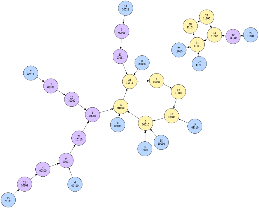
From this, it is easy to see that the circuit is fixpoint-free and the worst-case cycle length is four (the subgraph in the upper right corner).
Note that there is also a JSON output option. This is intended so that you can create a circuit template, run it through random mutations, simulate and evaluate it and automatically generate a file that is suitable for you as an exam or training question.
"mutate": Change Logisim circuits
The mutate command allows you to create a Logisim circuit, then change gates
in that circuit. It allows you, for example, to create a simple combinatorial
exercise question and randomly have gates swapped until a circuit comes out
that you like. Caveat: Logisim nets are based solely on their position -- it is
therefore imperative that where gates are swapped by longer counterparts, there
still needs to be at least one tiny piece of wire remaining. I.e., to be
completely safe use XNOR with all inverted inputs in your template everywhere
(it is the longest component) and do not place a source/component directly over
the XNOR pins, but at least have a piece of wire connect to it. Otherwise you
will encounter weird results (e.g., unconnected pins).
mutate works by specifying the template circuit along with a list of gate
labels to mutate along with a mutation specifier (i.e., what that gate should
be replaced by). If the mutation specifier is missing, all possible
combinations will be built (for a two-input gate, that is 24 combinations: AND,
OR, NAND, NOR, XOR, XNOR with no inverted inputs, inverted A, inverted B and
inverted A and B inputs makes 6 x 4 = 24. If two components are specified, that
number quickly grows (576 combinations for two components, 13824 for three,
etc.).
A mutation specifier is a comma-separated list which may contain the following items:
c=GATE: Allow this type of gate for replacement. If noc=directive is included in the mutation specifier, by default all six variants are included.inv=PINNO: Allow inversion of this pin number, count starting at 1. Ifinv=0is given this creates a mutation specifier in which no inputs are inverted at all.comb=INDEX: Select a specific combination out of the enumeration. For example, if nothing else is specified for a standard gate, this needs to be a number inbetween 0..23.randcomb=COUNT: SelectCOUNTrandom indices out of the pool of combinations.
For example, the following mutation specifiers are all valid (the text always assumes a two-input gate, but the syntax also works for gates with arbitrary number of inputs):
c=AND,c=OR: Replace only by AND or OR gates, all four input pin inversions possible.c=AND,index=0: Replace by AND gate with no pins inverted.c=AND,index=3: Replace by AND gate with both pins inverted.randcomb=1: Replace by a completely random gate with randomly inverted pins.c=XOR,c=NOR,inv=1: Replace by XOR and NOR with pin 1 either inverted or not (four combinations total).
For example, this command:
$ digtick mutate -m G1:randcomb=1 -m G2:randcomb=1 -m G3:c=AND examples/mutate_me.circ
Will generate 8 outputs files in the mutated-circuit directory. G1 and G2
are chosen fully random and all possible input pin variations of AND gates
are attempted for G3. Since G3 is a three-input gate, this makes for 8
possibilities.
Since the randcomb=1 selector is particularly useful, there is a handy shortcut:
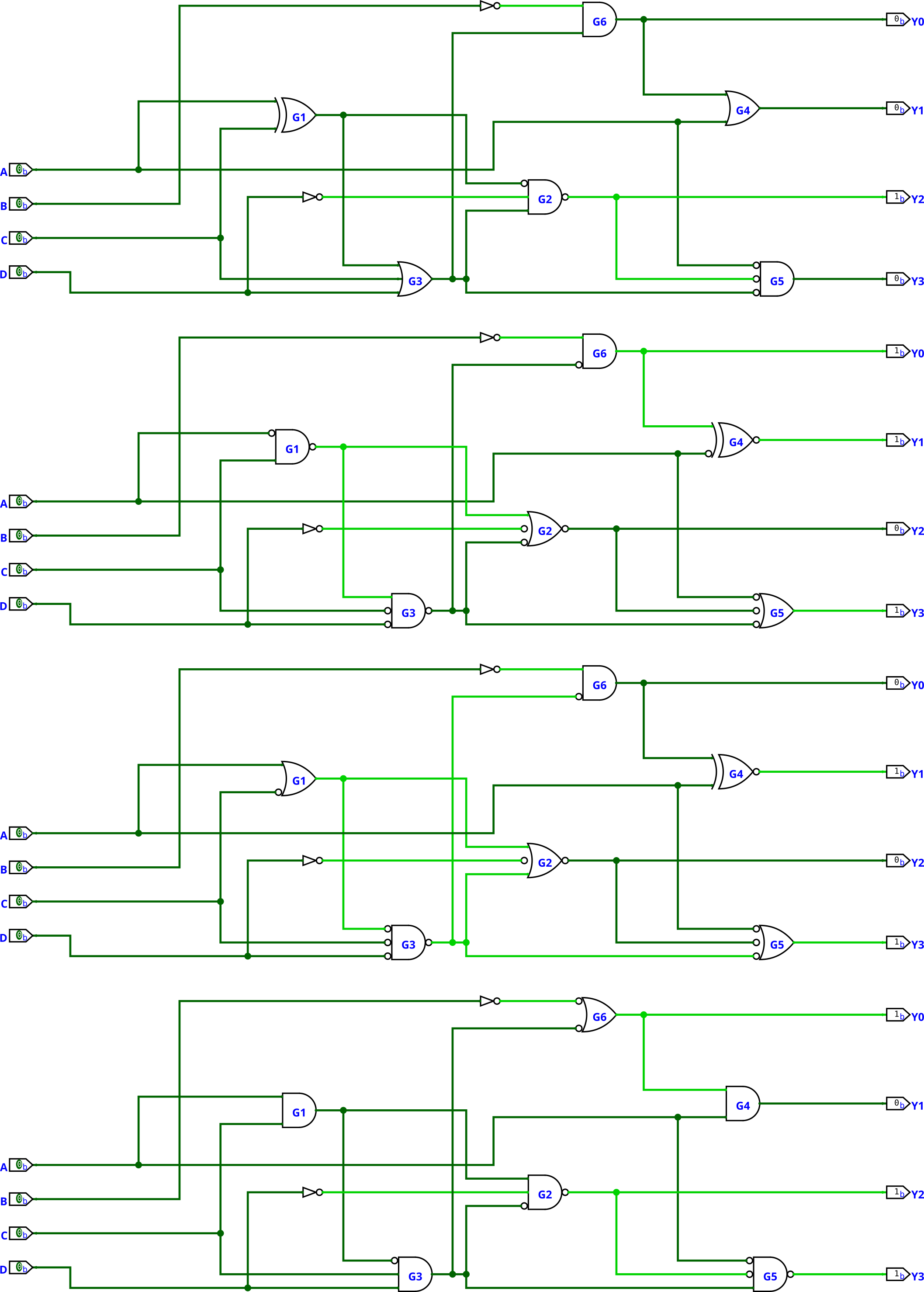
$ digtick mutate -r G1,G2,G3,G4,G5,G6 examples/mutate_me.circ
This creates only a single output file in which all of G1...G6 are fully
randomized (both in what components they are replaced by and which input pins
of theirs are inverted). This is the result when run four times in a row,
stacked on top of each other for easier comparison:
License
GNU GPL-3.


Download files
Download the file for your platform. If you're not sure which to choose, learn more about installing packages.
Source Distribution
File details
Details for the file digtick-0.1.0.tar.gz.
File metadata
- Download URL: digtick-0.1.0.tar.gz
- Upload date:
- Size: 152.1 kB
- Tags: Source
- Uploaded using Trusted Publishing? No
- Uploaded via: twine/6.1.0 CPython/3.13.7
File hashes
| Algorithm | Hash digest | |
|---|---|---|
| SHA256 |
9b29aaf65e509cfd62942e9d5d7092fe1c3381757ee44151be08ddad72c550eb
|
|
| MD5 |
26f236bb7968ef4c59a286094c1b4baa
|
|
| BLAKE2b-256 |
305e363365c38caaded65a7f8f28eebce91d44ee485f0a589ede99de0f8f8ddd
|


