
do-attribution
Multi-touch attribution and experimental calibration for Python — closed-form Markov, exact Shapley, temporal attribution, and explicit calibration from external lift-test evidence.


do-attribution has two explicit layers:
journey data        → attribution
external experiment → post-attribution calibration
The attribution layer turns customer journeys such as
"Email > Social > Purchase" and a 0/1 conversion flag per journey into
raw per-channel model diagnostics and, when those values satisfy the
normalization contract, per-channel shares using two observational
allocation models:
- an absorbing-Markov-chain removal-effect model
(
MarkovAttribution, orders 1+, four removal strategies), and - a cooperative-game Shapley-value model (
ShapleyAttribution, exact factorial weights over the observed coalition lattice).
The calibration layer applies caller-supplied lift-test evidence after a static or temporal attribution fit. Direct adjustments to tested entities, residual allocation to other entities, temporal evidence schedules, and provenance remain separate and inspectable.
Around these layers the package ships side-by-side model comparison
(CompareAttribution), explicit conversion-endpoint handling
(conversion_labels), plain-text reporting (summary()), flat DataFrame
export (to_dataframes()), matplotlib/networkx visualizations, and temporal
epoch analysis (TemporalMarkovAttribution, TemporalShapleyAttribution,
recommend_epochs) that refits the same static models independently inside
chronological epochs.
Scope guard: attribution outputs are probabilistic decompositions of observed co-occurrence between channel exposure and conversion — not causal inference. A high share means the model assigned relatively more normalized attribution to the channel from the observed paths; it does not identify the channel that caused a conversion. Calibration can apply external experimental evidence, but it does not convert attribution internals into causal effects or replace sound experimental design.
Key capabilities
- Deterministic, closed-form Markov attribution. Removal effects come
analytically from the absorbing-chain fundamental matrix
(I − Q)⁻¹— no Monte Carlo, no seed, no simulation count. Identical inputs always produce identical outputs. - Four removal-effect definitions.
removal_strategy="fail","fail_refit"(signed effects),"detour"(signed effects), or"redirect_to_null"— four operational meanings of "remove this channel", selected explicitly instead of implied. - Exact Shapley values. Per-channel values use the exact factorial weight
w(s, n) = s!·(n−s−1)!/n!. Raw signed values and the coalition value function are always returned; normalized shares are returned when the raw values admit a valid share vector, and reported as unavailable when they do not. - Conservation and contract guarantees. When normalized attribution is
available its shares are finite, lie on
[0, 1], and sum to 1, and attributed conversions conserve the observed total. When it is not,attributionisNonewith a machine-readable status and reason rather than a fabricated share vector.redirect_to_nullremoval effects are nonnegative by construction, and absorption probabilities stay on[0, 1]— enforced by the implementation. - Model reporting. Every fitted model renders a compact ASCII
summary()or a natural-languagesummary(output_format="report")— plain Python strings with bounded, distilled detail tables (signed removal effects, top transitions and drop-offs, top coalitions, path diagnostics). - Flat DataFrame export. Temporal models expose
to_dataframes() -> dict[str, pd.DataFrame]: flat, string-keyed, Parquet/SQL-ready tables for attribution, raw model values, and sample diagnostics — no text parsing, noMultiIndex, no lazy refits. - Visualization.
plot_attribution,plot_removal_effects,plot_transition_graph,plot_coalition_values,plot_attribution_comparison, andplot_epoch_recommendationeach return amatplotlib.figure.Figure. - Temporal epoch analysis. Calendar buckets (
freq=), explicit labels (fit_by_epoch), or data-driven boundaries (recommend_epochs+fit_recommended) — every epoch is an independent static fit; complete paths are never split across epochs. - Experimental calibration. Apply externally supplied lift-test evidence to static or fixed-epoch attribution results while keeping direct test adjustments, residual allocation, evidence schedules, epoch-level reductions, and provenance explicitly separate.
- Calibration diagnostics. One static adjustment-decomposition plot and six temporal diagnostics show evidence alignment, ratio construction, direct adjustments, residual allocation, entity mix, and evidence strength.
- Reproducible outputs. Deterministic model fits, deterministic renderers, and deterministic tie ordering — identical inputs always produce identical reports, tables, and figures.
Core runtime dependencies are numpy and pandas.
Installation
pip install do-attribution
| Extra | Installs | Enables |
|---|---|---|
viz |
matplotlib, networkx |
all plotting helpers |
temporal |
statsmodels, ruptures |
global-signal epoch recommendation |
excel |
openpyxl |
Excel-friendly workflows |
dev |
all of the above + pytest |
running the test suite |
pip install "do-attribution[viz]"
pip install "do-attribution[temporal,viz]"
Requires Python 3.10 or newer.
Quick start
A complete, runnable analysis — ten journeys, a fitted Markov model, shares, and a readable report:
from do_attribution import MarkovAttribution

journeys = [
    "Email > Social > Purchase",
    "Search > Email > Purchase",
    "Social > Purchase",
    "Email > Search",                       # no conversion
    "Search > Social > Email > Purchase",
    "Direct > Purchase",
    "Email > Social",                       # no conversion
    "Search > Email > Social > Purchase",
    "Social > Email > Purchase",
    "Search",                               # no conversion
]
conversions = [1, 1, 1, 0, 1, 1, 0, 1, 1, 0]

model = MarkovAttribution(
    order=1,
    removal_strategy="redirect_to_null",
    conversion_labels=["Purchase"],   # endpoint token, not a channel
    return_transition_matrix=True,
)
result = model.fit(journeys, conversions)

print({ch: round(share, 4) for ch, share in result["attribution"].items()})
print(f"P(conversion | start) = {result['total_conversion_probability']:.4f}")
print(model.summary())
Output (abridged — the summary continues with top transitions, drop-off bottlenecks, and path diagnostics):
{'Direct': 0.085, 'Email': 0.3912, 'Search': 0.1913, 'Social': 0.3324}
P(conversion | start) = 0.7000
Attribution Summary
Model: MarkovAttribution
Epoch source: static
Overall: 10 paths, 7 conversions, 70.00% conversion rate

Data
+-----------+-------+-------------+---------+--------------------------------------------+
| Cohort    | Paths | Conversions | Conv. % | Top channels                               |
+-----------+-------+-------------+---------+--------------------------------------------+
| All paths | 10    | 7           | 70.00%  | Email 39.12%, Social 33.24%, Search 19.13% |
+-----------+-------+-------------+---------+--------------------------------------------+

Removal effects (raw, signed) vs normalized shares
+---------+----------------+--------+
| Channel | Removal effect | Share  |
+---------+----------------+--------+
| Email   | +0.6571        | 39.12% |
| Social  | +0.5584        | 33.24% |
| Search  | +0.3214        | 19.13% |
| Direct  | +0.1429        | 8.50%  |
+---------+----------------+--------+
The Shapley model is a drop-in alternative on the same inputs. Note that
attribution may be None — always check before indexing it:
from do_attribution import ShapleyAttribution

shapley = ShapleyAttribution(conversion_labels=["Purchase"]).fit(journeys, conversions)

if shapley["attribution"] is None:
    print(shapley["normalization_status"], shapley["normalization_reason"])
    # unavailable near_cancellation
    print({ch: round(v, 4) for ch, v in shapley["shapley_values"].items()})
    # {'Direct': -0.5833, 'Email': 0.25, 'Search': -0.0833, 'Social': 0.4167}
else:
    print({ch: round(share, 4) for ch, share in shapley["attribution"].items()})
On this dataset no journey touches all four channels, so v(N) = 0, the raw
values cancel to float residue, and no valid share vector exists. The model
reports that rather than dividing by the residue. The raw signed values are
still returned — they are diagnostics on the game's own scale, not shares.
Lists, NumPy arrays, and pandas Series all work as path and conversion inputs.
Visual examples
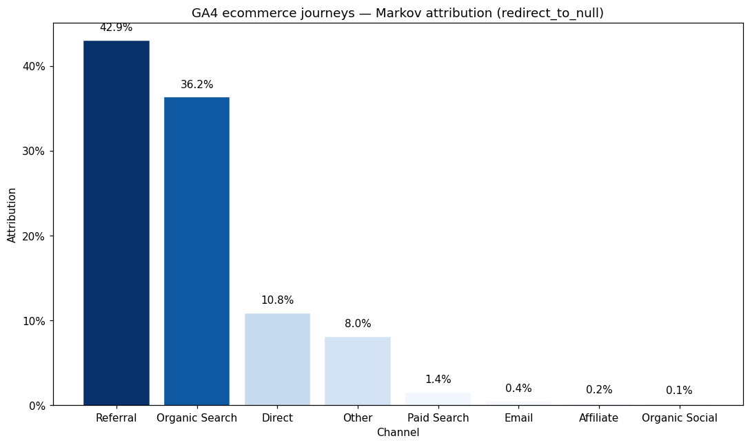
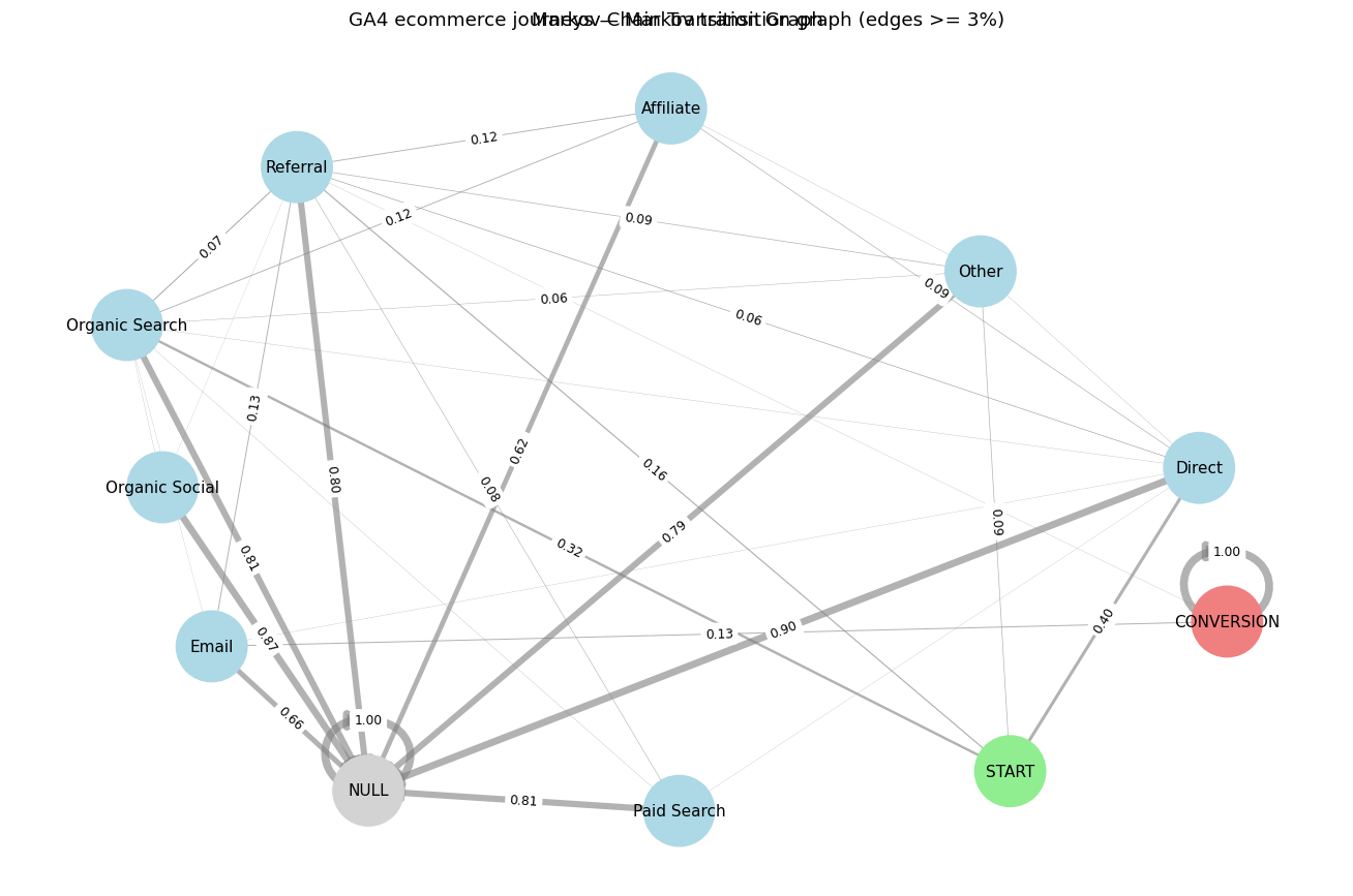
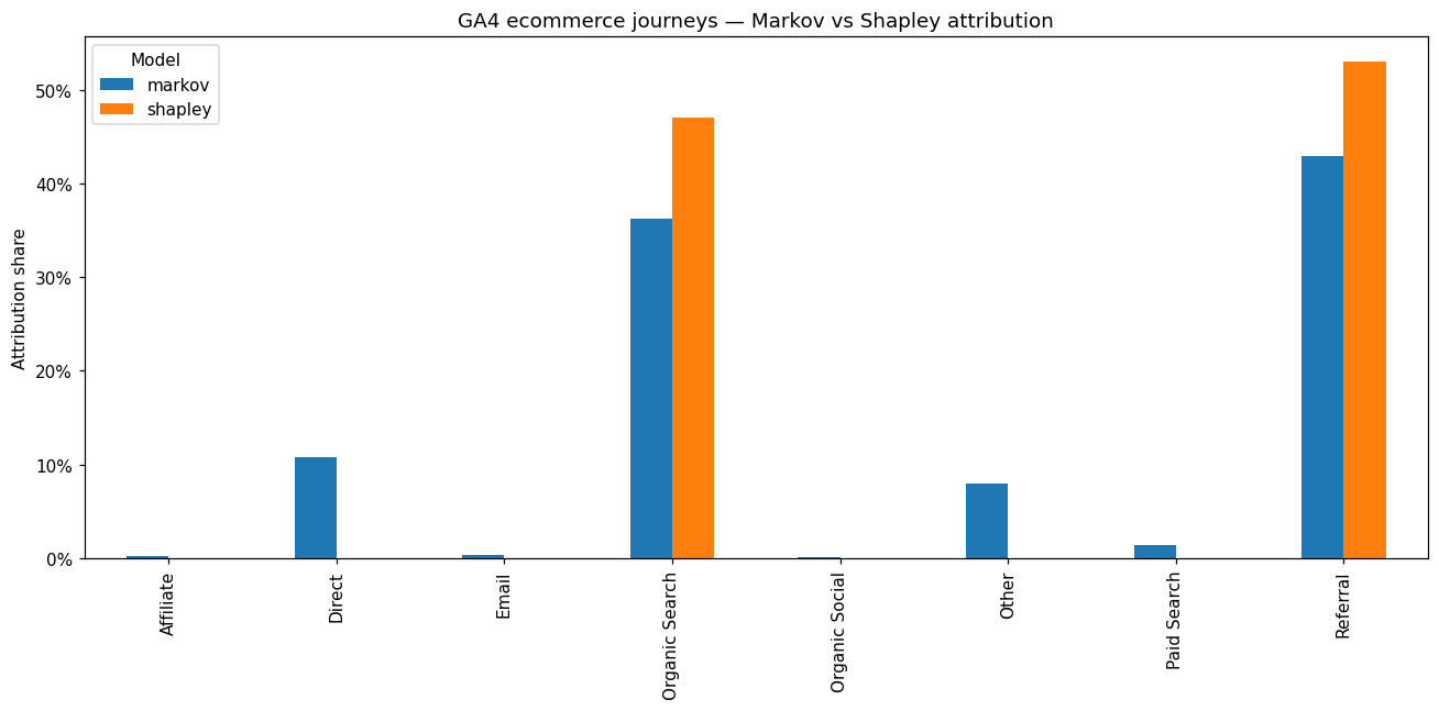
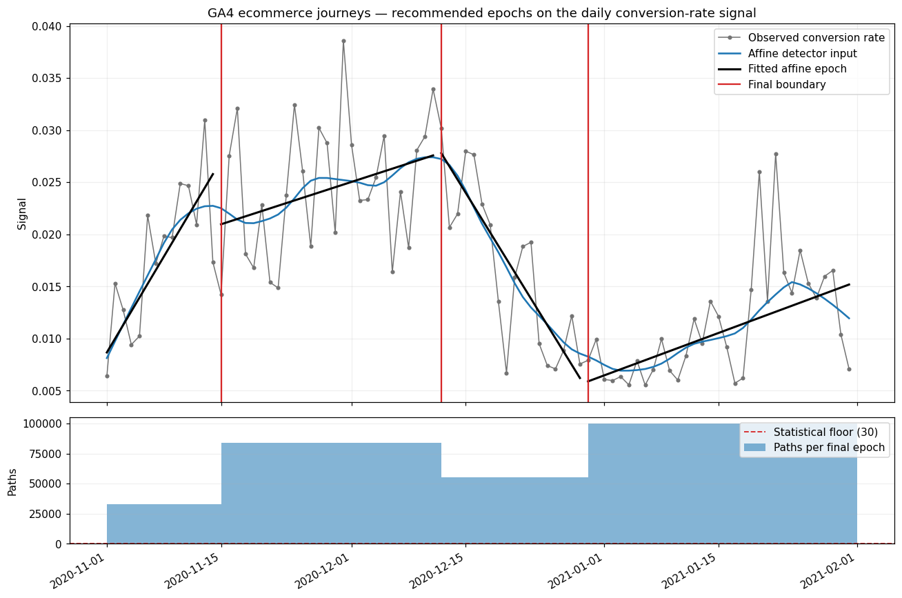
The GA4 ecommerce example shows how the package allocates attribution across channels, represents journey transitions, compares model outputs, and identifies candidate temporal boundaries.
 |
 |
plot_attribution — Markov attribution shares by channel |
plot_transition_graph — fitted journey transitions with edges ≥ 3% |
 |
 |
plot_attribution_comparison — Markov and Shapley attribution on the same journeys |
plot_epoch_recommendation — candidate and retained epoch boundaries on the conversion-rate signal |
Calibration diagnostics keep experimental evidence, constructed calibration ratios, direct adjustments, and policy-based residual allocation visually distinct.
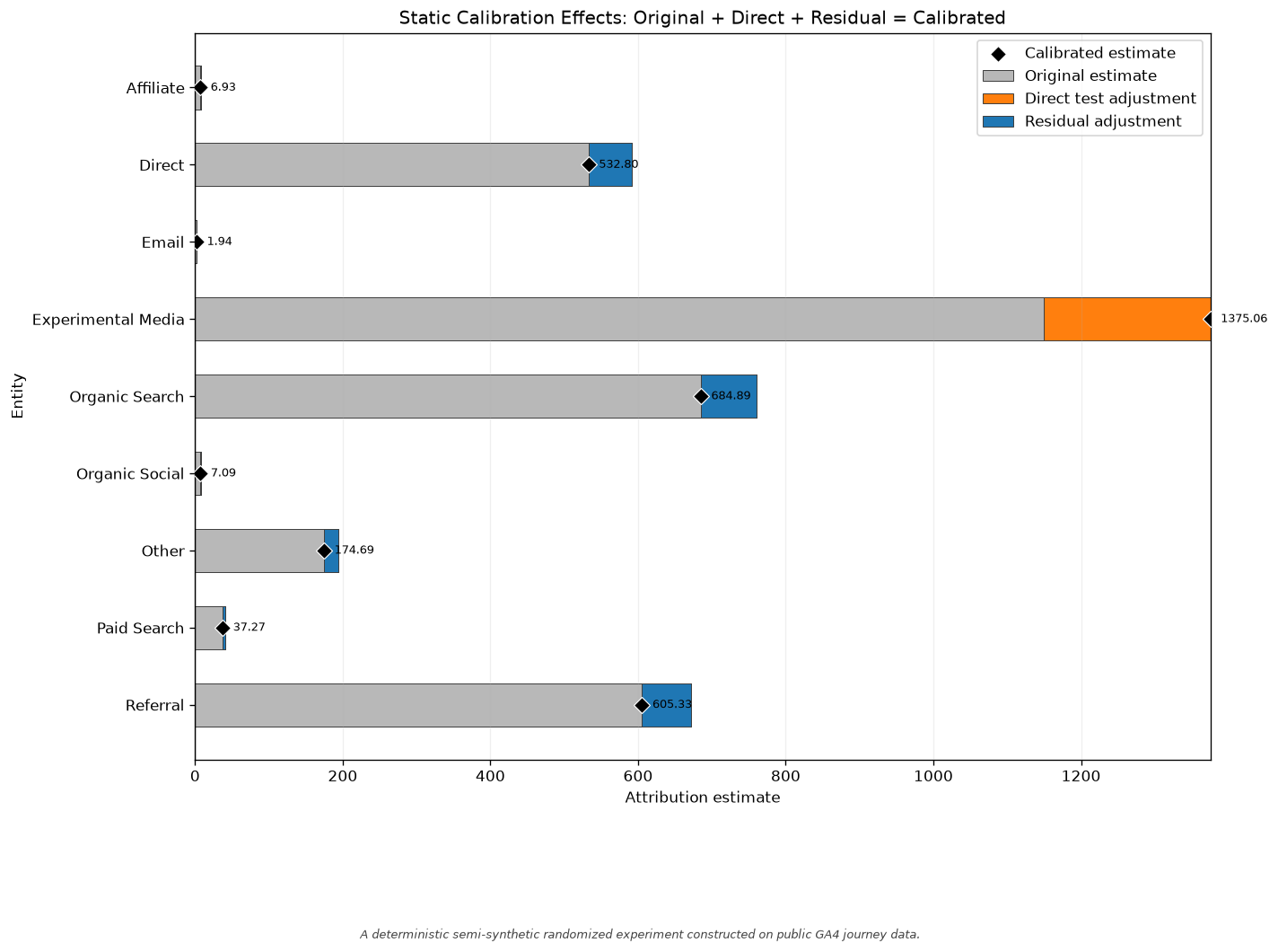 |
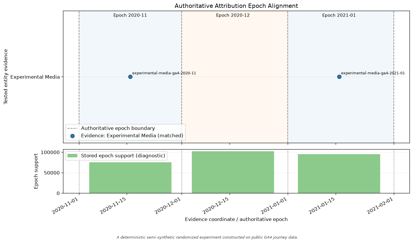 |
| Decomposes the calibrated estimate into original attribution, direct test adjustment, and residual allocation | Shows where experimental evidence falls on caller-defined epochs without redefining the epoch boundaries |
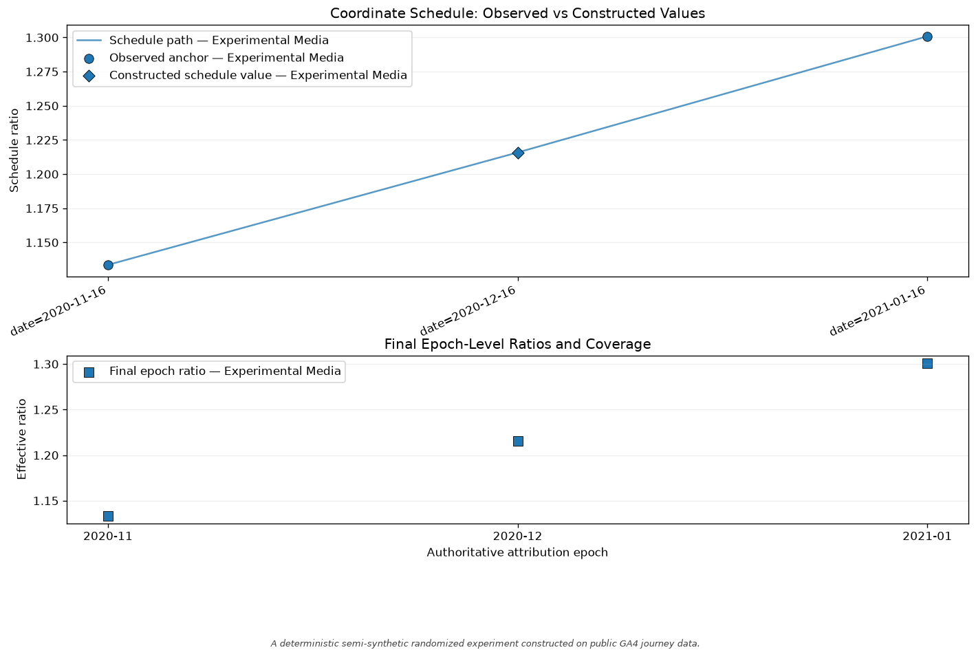 |
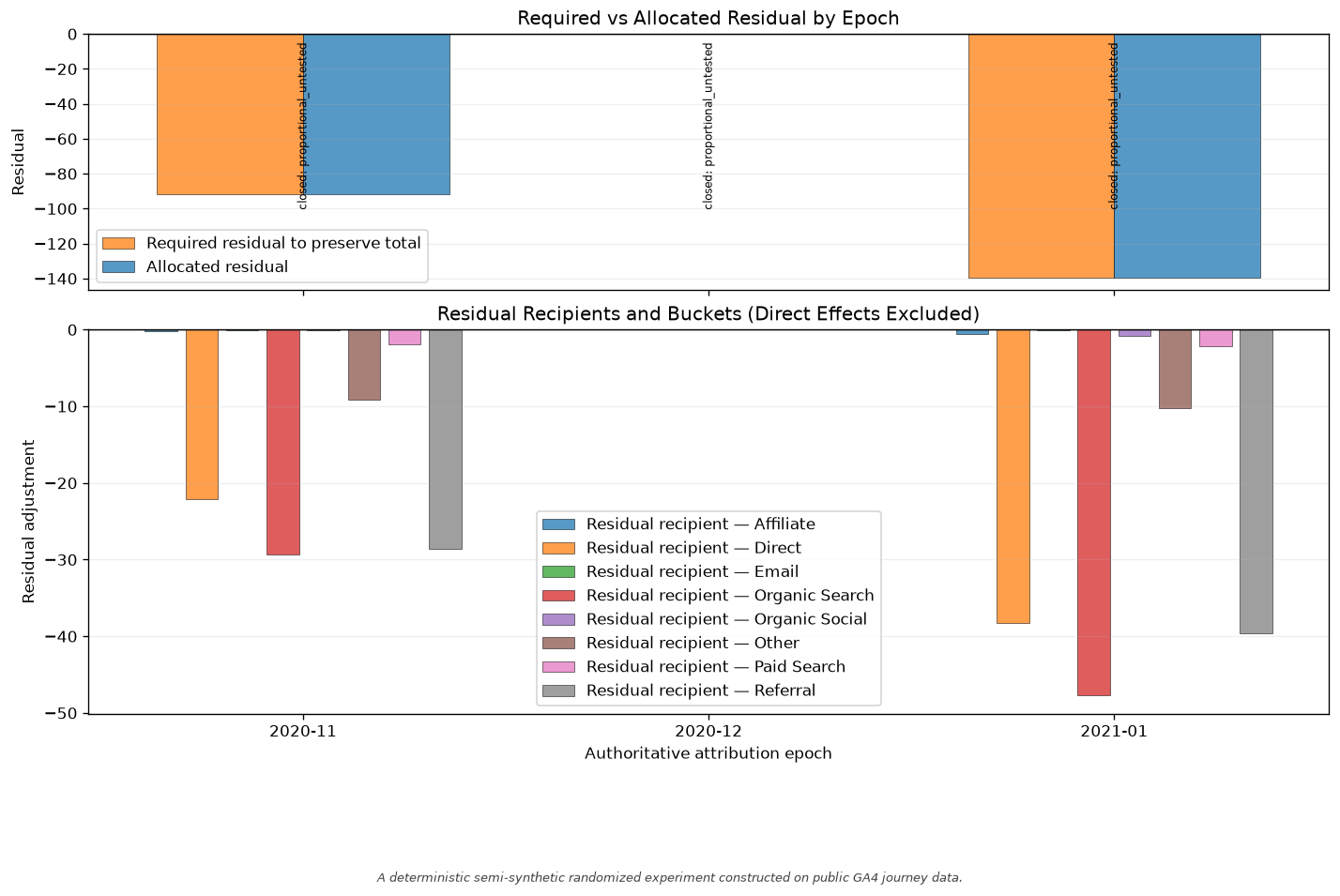 |
| Distinguishes observed experimental anchors from constructed epoch-level calibration ratios | Shows the required residual adjustment and its policy-based allocation across eligible recipients |
Experimental calibration
LiftTestEvidence represents external experimental evidence for one tested
entity: an observed lift and the attribution estimate matched to the same
population, outcome, and window, plus identifying metadata and optional
uncertainty and temporal coordinates. Its calibration ratio is:
calibration ratio = observed lift / matched attribution estimate
Optional standard_error is validated and retained on the
LiftTestEvidence record as experimental evidence metadata and provenance.
Deterministic point calibration does not use or propagate it: changing
standard_error does not change the calibration ratio, direct adjustment,
residual allocation, or calibrated total.
Calibrated point outputs therefore do not supply confidence intervals,
posterior uncertainty, or uncertainty-adjusted calibration ratios.
AttributionCalibration applies that evidence to caller-approved static
attribution estimates. TemporalAttributionCalibration applies dated
evidence to estimates on a caller-supplied, authoritative epoch grid; the
evidence coordinates do not redefine the epochs.
Every static application requires an explicit residual policy. Every temporal application additionally requires an explicit ratio policy and epoch-ratio policy. The result keeps the tested entity's evidence-backed direct adjustment separate from any residual allocated to untested entities. Those recipient changes are policy allocations, not effects measured by the experiment. Interpolated schedule values and constant-policy values transported to declared epochs are constructed values, not new experimental observations.
This runnable example uses the full-period values and evidence identity from the calibration notebook:
from do_attribution import AttributionCalibration, LiftTestEvidence

attributed_conversions = {
    "Experimental Media": 1149.1519,
    "Organic Search": 760.3327,
    "Referral": 672.0069,
    "Direct": 591.4872,
    "Other": 193.9282,
    "Paid Search": 41.3767,
    "Organic Social": 7.8723,
    "Affiliate": 7.6895,
    "Email": 2.1544,
}

evidence = LiftTestEvidence(
    tested_entity="Experimental Media",
    observed_lift=1375.0555,
    matched_mta_estimate=attributed_conversions["Experimental Media"],
    test_id="experimental-media-ga4-full-eligible-period",
    outcome_name="journey conversion",
)

calibration = AttributionCalibration([evidence])
calibrated = calibration.apply_estimates(
    estimates=attributed_conversions,
    residual_policy="proportional_untested",
    eligible_entities=[
        entity
        for entity in attributed_conversions
        if entity != evidence.tested_entity
    ],
)

print(calibrated.summary())
figure = calibrated.plot_calibration_effects()
Calibration consumes attribution estimates that the caller has already reviewed and approved. It does not reinterpret Markov removal effects, Shapley values, or other attribution internals as causal effects, and it does not choose the experiment, matching design, or calibration policies for the caller.
See docs/calibration.md
for the policy contract,
docs/calibration_examples.md
for static
examples, and
docs/calibration_examples_temporal.md
for temporal schedules and epoch reduction.
Supported attribution methods
Markov removal-effect attribution
MarkovAttribution(order=k) models journeys as an absorbing Markov chain
(START, channels or sliding k-tuples of channels, CONVERSION, NULL)
and credits each channel by its removal effect, computed in closed form.
Four operational definitions of removal are provided:
| Strategy | Population | Behavior | Raw-effect sign contract |
|---|---|---|---|
"fail" |
Fixed: every original journey and weight is retained. | Strip the channel, force affected conversions to failure, rebuild the chain, and recompute P(CONVERSION | START). |
No blanket sign guarantee; normalization is returned only when the shared share contract succeeds. |
"fail_refit" |
Refit: only usable transformed journeys remain, so count and total weight may change. | Preserve the legacy strip-and-refit procedure under an explicit name. | Signed. |
"detour" |
Refit after trimming; the usable population may change if trimming empties paths. | Strip the channel while retaining original conversion flags, then refit. A negative effect means removing the channel lowered modelled conversion probability. | Signed. |
"redirect_to_null" |
Fixed fitted transition matrix; no journey refit. | Redirect the removed channel's transition mass to NULL on the fitted matrix and recompute absorption analytically — the classic removal-effect definition. |
Nonnegative by construction. |
Under fixed-population "fail", removing the selected channel can leave a
journey with no modeled channel states. That journey is retained with its
original weight as an explicit START -> NULL failure; it is never silently
discarded.
"fail_refit" keeps the previous strip-and-refit procedure: emptied
transformed paths are dropped before the chain is rebuilt. The transformed
journey count and total weight can therefore be smaller than the originals,
so its result answers a different population question from "fail".
result["population_diagnostics"] reports both counts, both total weights,
the number of emptied and dropped paths, and the empty-path rule for every
removed channel.
Migration is explicit when preserving the previous behavior:
paths = ["A"] * 4 + ["B"] * 4
converted = [1, 1, 1, 0, 1, 0, 0, 0]

fixed = MarkovAttribution(removal_strategy="fail").fit(paths, converted)
legacy_refit = MarkovAttribution(
    removal_strategy="fail_refit"
).fit(paths, converted)

fixed["population_diagnostics"]["A"]["transformed_journey_count"]         # 8
legacy_refit["population_diagnostics"]["A"]["transformed_journey_count"]  # 4
Raw effects from fail, fail_refit, and detour are diagnostics rather
than probabilities. Signed effects from fail_refit or detour do not
necessarily define a probability distribution and must not be interpreted as
percentages. The model normalizes raw effects only when they satisfy the
shared finite, nonnegative, bounded, unit-sum contract. If signed effects
cancel at or below the scale-aware tolerance, attribution is None;
normalization_status, normalization_reason, and the raw-sum, magnitude,
denominator, and cancellation-ratio diagnostics explain why while
removal_effects remain available.
Higher orders (order=2, order=3, …) use sliding tuples as states; short
paths are left-padded with START. fit returns attribution,
removal_effects, total_conversion_probability, and (opt-in) the
transition_matrix.
Shapley coalition attribution
ShapleyAttribution uses the value function v(S) = conversions on paths
whose unique channel set is exactly S and exact factorial weights. fit
returns attribution, raw signed shapley_values, and the observed
value_function:
shapley["value_function"]
# {('Email', 'Social'): 2, ('Email', 'Search'): 1, ('Social',): 1, ...}
Raw signed shapley_values and normalized attribution are separate
outputs with separate contracts:
| Output | Contract |
|---|---|
shapley_values |
Always present. Signed, on the game's own scale. Not shares, percentages, or probabilities. |
attribution |
A share mapping when available, otherwise None. Every value is finite and in [0, 1], and the values sum to 1. |
Because no journey may touch every channel, the efficiency axiom forces the
raw values to sum to v(N) = 0 by construction. Dividing by that float
residue produces numerically explosive output, so normalization is refused
instead: attribution is None, a warning is emitted, and the fit still
succeeds with its raw values and diagnostics intact.
shapley["normalization_status"]      # 'available' | 'unavailable'
shapley["normalization_reason"]      # e.g. 'near_cancellation'
shapley["raw_sum"]                   # ~1e-17 — float residue, not a real total
shapley["raw_magnitude"]             # 1.3333
shapley["cancellation_ratio"]        # ~1e-17 — far below the 1e-12 threshold
The exact residue in raw_sum is not reproducible across summation orders,
which is precisely why the scale-aware ratio, rather than the bare sum, drives
the decision.
Normalization is unavailable when the raw magnitude is zero, when the
scale-aware cancellation ratio |Σrᵢ| / Σ|rᵢ| falls at or below 1e-12, or
when the candidate shares leave [0, 1] or fail to sum to 1. The reason
codes are zero_raw_magnitude, near_cancellation, nonfinite_result,
negative_share, share_above_one, and invalid_share_sum.
Attributed conversions are only defined when attribution is available;
they are never derived from raw signed values.
Side-by-side comparison
from do_attribution import CompareAttribution

comparison = CompareAttribution(conversion_labels=["Purchase"])
comparison.fit(journeys, conversions)

comparison.attribution_frame()      #           markov  shapley
                                    # Direct  0.026316      NaN
                                    # Email   0.394737      NaN
                                    # Search  0.201754      NaN
                                    # Social  0.377193      NaN
comparison.unavailable_models()     # {'shapley': 'near_cancellation'}
comparison.difference_frame("markov")
The two methods answer different statistical questions and can disagree
materially without either being defective — difference_frame makes the
disagreement explicit. extra_models={...} plugs any additional
BaseAttribution implementation into the same aligned tables, so
first-touch, last-touch, or any custom baseline can sit beside the two
built-in models.
Conversion-endpoint declaration
Terminal outcome tokens ("Purchase", "Sale", …) are declared, not
guessed: conversion_labels=["Purchase"] strips them before channel
extraction, state construction, coalition enumeration, reporting, and
plotting. Labels colliding with the reserved START/CONVERSION/NULL
tokens raise ValueError; conversion_labels=None treats every token as a
channel.
Temporal epoch analysis
TemporalMarkovAttribution and TemporalShapleyAttribution are
chronological orchestrators: each complete path is assigned to exactly one
epoch by a single anchor timestamp, each epoch gets an independent static
fit, and adjacent epochs share nothing — jumps at boundaries are valid
outputs of a discontinuous piecewise model, not smoothing artifacts.
import pandas as pd
from do_attribution import TemporalShapleyAttribution

anchors = pd.to_datetime([
    "2025-01-05", "2025-01-12", "2025-02-08", "2025-02-17", "2025-04-03",
    "2025-04-21", "2025-07-09", "2025-07-19", "2025-10-02", "2025-10-18",
])

by_quarter = TemporalShapleyAttribution(
    freq="Q",                      # calendar buckets; per-year mappings supported
    min_samples_per_epoch=1,       # demo-sized floor
    conversion_labels=["Purchase"],
)
by_quarter.fit(journeys, anchors, conversions)

by_quarter.get_trend("Email")             # share by epoch; NaN where unavailable
tables = by_quarter.to_dataframes()       # flat DataFrames, ready for Parquet/SQL
list(tables)
# ['attribution', 'shapley_values', 'epoch_summary', 'channel_epoch_sample_sizes']
The Markov variant additionally exports removal_effects,
conversion_probability, and transition_matrices tables. Three entry
points cover epoch selection:
fit(paths, timestamps, conversions)— calendar frequency buckets;fit_by_epoch(paths, epoch_labels, conversions)— explicit labels;fit_recommended(paths, conversions, anchor_timestamps)— data-driven boundaries fromrecommend_epochs, which segments a global daily conversion-rate signal with a penalized piecewise-affine detector (weekly/multi-seasonal STL decomposition, robust second-difference scale with serial-correlation correction, PELT with a custom weighted affine cost), enforces minimum epoch width and path-count floors, and returns auditable left-closed, right-open boundaries. A Markov-onlysignal="transition_drift"variant segments aligned order-1 transition matrices.plot_epoch_recommendationrenders the fitted segment geometry, kept and rejected knots, and per-epoch path counts.
Sample-size diagnostics (get_epoch_summary,
get_channel_epoch_sample_sizes, order- and strategy-aware effective
floors, and the suggest_freq calendar sanity check) flag thin epochs
before you interpret an adjacent-epoch jump. After fitting,
detect_threshold_crossings(channel, threshold=...) returns adjacent
epoch changes whose absolute delta exceeds the caller-supplied threshold.
This is a descriptive comparison, not a statistical test.
detect_significant_changes(...) remains temporarily available as a
deprecated compatibility alias.
Reporting and export
Every fitted model — static, temporal, or a standalone recommendation — renders deterministic plain text:
print(model.summary())                          # compact ASCII tables
print(model.summary(output_format="report"))    # natural-language narrative
Summaries distill rather than dump: bounded top-k detail tables (signed
removal effects, top transitions and drop-offs, top coalitions, path
diagnostics) with the complete grids available programmatically via
to_dataframes() and the get_* accessors. The reporting language is
descriptive; it never labels a movement statistically significant or causal.
Detailed examples
All six notebooks run end to end on the same GA4 journey extract
(examples/ga4_attribution_journeys.csv)
— a transformed journey-level
extract created from
Google's public obfuscated GA4 ecommerce sample
(Google Merchandise Store): one row per journey with an ordered channel
path, a binary conversion flag, and an anchor timestamp.
| Example | Shows |
|---|---|
examples/basic_markov.ipynb |
static Markov fit, shares, removal effects, summary, transition graph |
examples/basic_shapley.ipynb |
Shapley shares, raw values, coalition results, coalition plot |
examples/side_by_side.ipynb |
CompareAttribution aligned tables, differences, comparison plot |
examples/temporal_markov.ipynb |
weekly Markov epochs, diagnostics, to_dataframes(), epoch recommendation |
examples/temporal_shapley.ipynb |
weekly Shapley epochs, channel trends, diagnostics, epoch recommendation |
examples/attribution_experiment_calibration.ipynb |
seeded semi-synthetic randomized campaign on the GA4 rows, matched static and temporal Markov estimates, calibration, and seven diagnostics |
Project status
do-attribution is in pre-1.0 development. The public API may change before
version 0.1.
License and attribution
MIT © 2026 Aaron Goodin — see
LICENSE.
The bundled example dataset and the figures generated from it derive from Google's public obfuscated GA4 ecommerce sample (Google Merchandise Store), transformed into a journey-level extract for demonstration. The calibration example additionally uses deterministic semi-synthetic randomized campaign assignment and lift-test outcomes generated by this project; those experimental variables are not part of Google's source dataset. Attribution outputs describe statistical association under each model's assumptions; they are not causal effect estimates.
1 maintainer

Metadata
1 maintainer
Release files for do-attribution 0.0.2
For a detailed explanation of source distributions (sdists) and built distributions (wheels), please see the package formats documentation.
Source distribution (sdist)
| File | Size | Uploaded | |
|---|---|---|---|
| do_attribution-0.0.2.tar.gz | 6.5 MB | Details |
Built distribution (wheel)
| File | Interpreter | ABI | Platform | Reset |
|---|---|---|---|---|
| do_attribution-0.0.2-py3-none-any.whl | Python 3 | none | any | Details |
Total release size: 6.6 MB
Release files / do_attribution-0.0.2.tar.gz
| Download URL | do_attribution-0.0.2.tar.gz |
|---|---|
| Size | 6.5 MB |
| Tags | Source |
|
SHA-256 checksum How to use checksums |
a909b6c3f1f3e04373ebb995b014948b9b62ff1f75106a50fa2a7b54b2689efe
|
|
BLAKE2b-256 checksum How to use checksums |
671ebe8806cc0bb8cb01876e0cd128f045e405ae60d1a0c6297194e9dc770028
|
| Upload date | |
|
Uploaded using Trusted Publishing? What is trusted publishing? |
No |
| Uploaded via |
twine/7.0.0 CPython/3.12.13
|
Release files / do_attribution-0.0.2-py3-none-any.whl
| Download URL | do_attribution-0.0.2-py3-none-any.whl |
|---|---|
| Size | 163.2 kB |
| Tags | Python 3 |
|
SHA-256 checksum How to use checksums |
793320da4a27e9549731543842a4643364c76183c6c292c30e803ab97fc229e5
|
|
BLAKE2b-256 checksum How to use checksums |
0b756cd61de08a4134d17dd83108725e78c2ffc7f5e1d5ffad5a0d11c3b4a1c9
|
| Upload date | |
|
Uploaded using Trusted Publishing? What is trusted publishing? |
No |
| Uploaded via |
twine/7.0.0 CPython/3.12.13
|














