
Double Sphere & multi-model spherical-camera platform: models, calibration, conversion & 3D for wide-FOV lenses
Verified details
These details have been verified by PyPIProject links
GitHub Statistics
Maintainers

Project description
DS-MSP — Double Sphere & Multi-model Spherical-camera Platform






A clean, tested, OpenCV-compatible platform for wide-FOV (fisheye / omnidirectional) cameras: a uniform multi-model layer — UCM, EUCM, Kannala-Brandt, RadTan, OCamCalib, Double Sphere, and the closed-form-invertible DS⁺ / EUCM⁺ — all behind one contract, with analytic Jacobians, intrinsics calibration, model conversion, two-view & stereo 3D, and hardware export. Built around the Double Sphere model (Usenko et al. 2018). It doubles as a guided, runnable course in wide-FOV camera geometry.
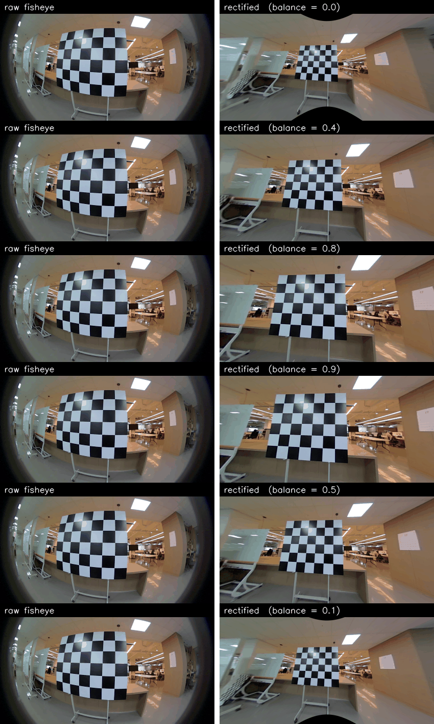
A real fisheye frame (left) rectified to a pinhole view (right), sweeping the
balanceknob from widest-FOV to tightest-crop. The bent ceiling lines and curved checkerboard straighten out.
Two ways in — pick yours:
- 🎓 Learn the geometry → start the runnable curriculum in
docs/learn/. Each chapter prints a number you can verify; the 🏆 capstone calibrates a real fisheye from TUM-VI footage and matches the published intrinsics to 0.003 % focal (0.08 px median).- 🛠️ Use the library → jump to Installation and Quick start.
Table of contents
- Why DS-MSP
- See the geometry
- Installation
- Quick start
- Repository map
- Learn: the guided curriculum
- Using the library
- Calibration
- Multi-camera rig calibration (MC-Calib-compatible)
- Deep dive: FOV, validity & undistortion
- Accuracy & verification
- FAQ
- Roadmap
- Credits
- License
Why DS-MSP
Fisheye lenses capture a very wide field of view — often > 180° — by deliberately bending straight
lines. The familiar pinhole model can't describe that, and worse, its X/Z projection blows up as
rays approach 90°. DS-MSP implements the models that can, and does it carefully:
| What you get | |
|---|---|
| Correct wide-FOV geometry | Double Sphere with the exact z > -w₂·d₁ half-space validity test — handles the full > 180° FOV, not the naive z > 0 check that silently clips it. |
| One interface, many models | UCM, EUCM, Kannala-Brandt (= OpenCV fisheye), RadTan (= OpenCV pinhole), OCamCalib, Double Sphere — plus closed-form DS⁺ / EUCM⁺ for lenses DS can't fit — all behind a single CameraModel contract. |
| Analytic Jacobians | Exact closed-form derivatives (no autodiff, no finite differences) → faster, more robust calibration. KB & RadTan match OpenCV to ~1e-13. |
| Model conversion | Translate a calibration between models without images or recalibration (sample → unproject → LM refit). |
| Calibration | Generic Levenberg–Marquardt bundle adjustment for any model, with a robust (Cauchy) loss option. |
| Multi-camera rigs | An MC-Calib-compatible rig pipeline (ds_msp.rig): one calib_param.yml, ChArUco images in, MC-Calib-format extrinsics out — with a different camera model per camera. (preview, from source → 0.8.0) |
| Ecosystem fluency | Read/write Kalibr camchain YAML and MC-Calib interchange; OpenCV-style drop-in API; TI Jacinto LDC hardware mesh export. |
| Verified, CI-tested | 426 tests + import-linter layer checks + mypy, green on Python 3.10–3.12. |
See the geometry
🎥 Prefer to drive it yourself? Open the live interactive studio → — pick any of the eight camera models the library ships, drag a 3D point, and step its projection onto a sphere, cylinder, or plane in real time. Every pixel is computed by a TypeScript port of
ds_msp, cross-checked against the library to ~10⁻¹² px. Source lives inweb/; it stays in the repo but never ships withpip install ds-msp.
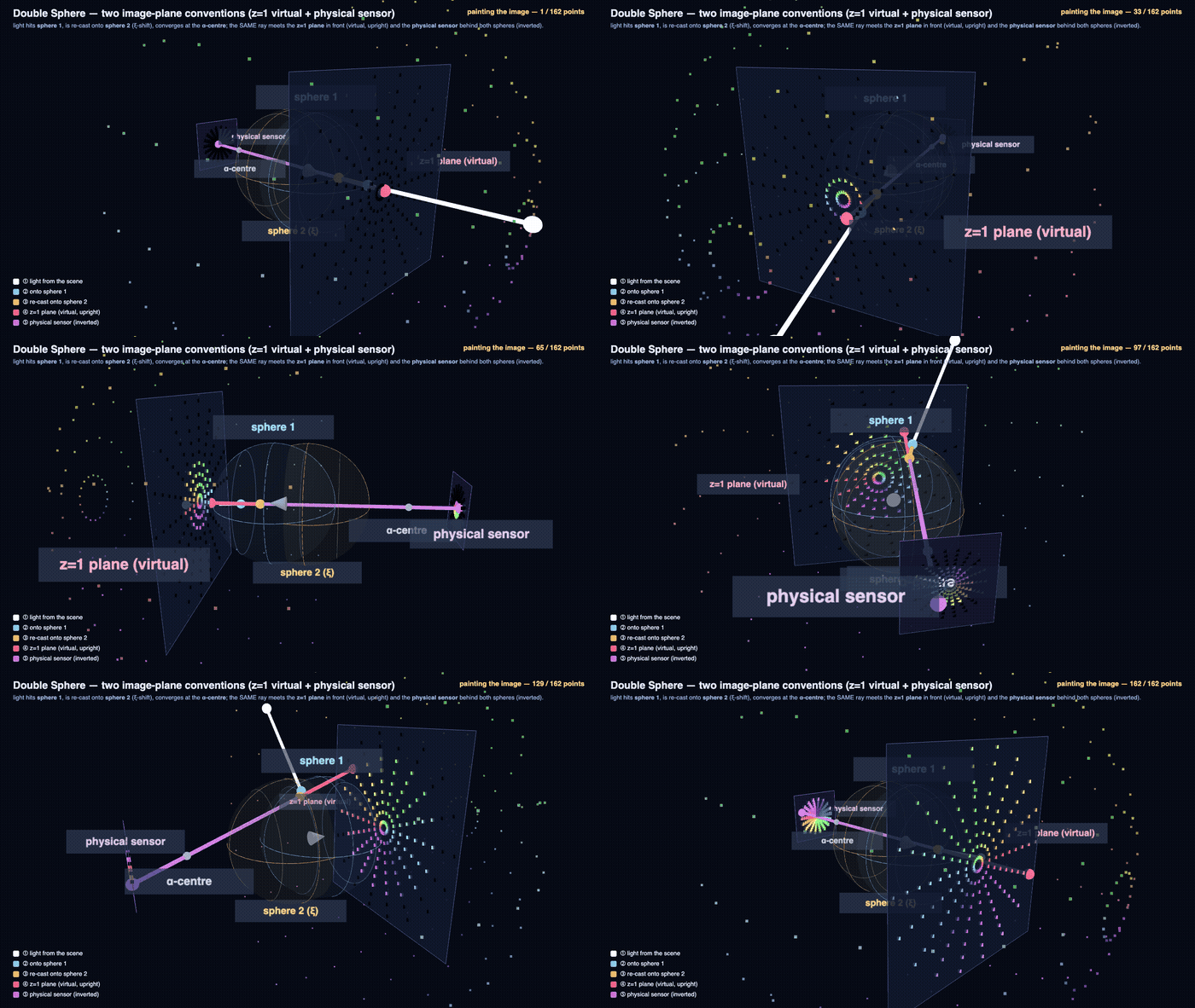
A camera model is a recipe for turning 3D rays into pixels. Here the Double Sphere model
runs on a synthetic scene — each world point is traced through its two spheres and projected
from the α-centre, painting the fisheye image point by point. One projection ray meets both
image-plane conventions at once: the model's normalized z = 1 plane (the virtual, upright
image the equations use) and the physical sensor behind both spheres (the real, inverted
image). The render's geometry is cross-checked against the library itself (std = 2e-16), so the
animation can't drift from the math:
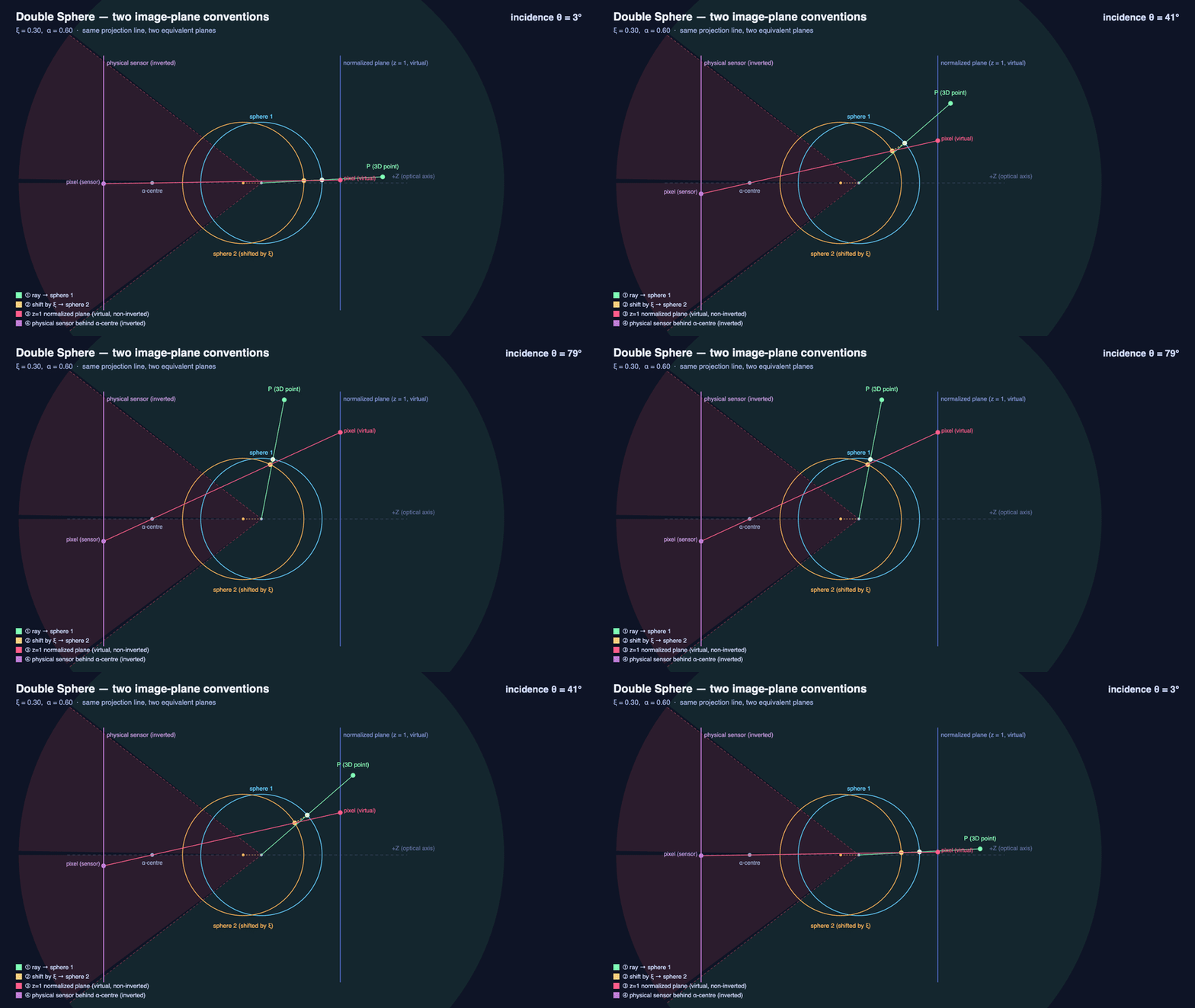
The Double Sphere is radially symmetric, so a single 2-D cross-section tells the whole story — here the same construction with both image planes labelled (the two spheres lie between the 3-D world and the sensor, exactly as in the paper):
And the image doesn't have to live on a flat plane. Because a fisheye is fundamentally a map from rays to pixels, those rays can be stored equally on a sphere, a cylinder, or a pinhole plane — and you can convert pixels between the three with exact, invertible math (round-trips to 1e-13 px). The sphere is the complete model; the flat pinhole is the awkward special case that can't hold a >180° view. Watch one real fisheye morph through all three:
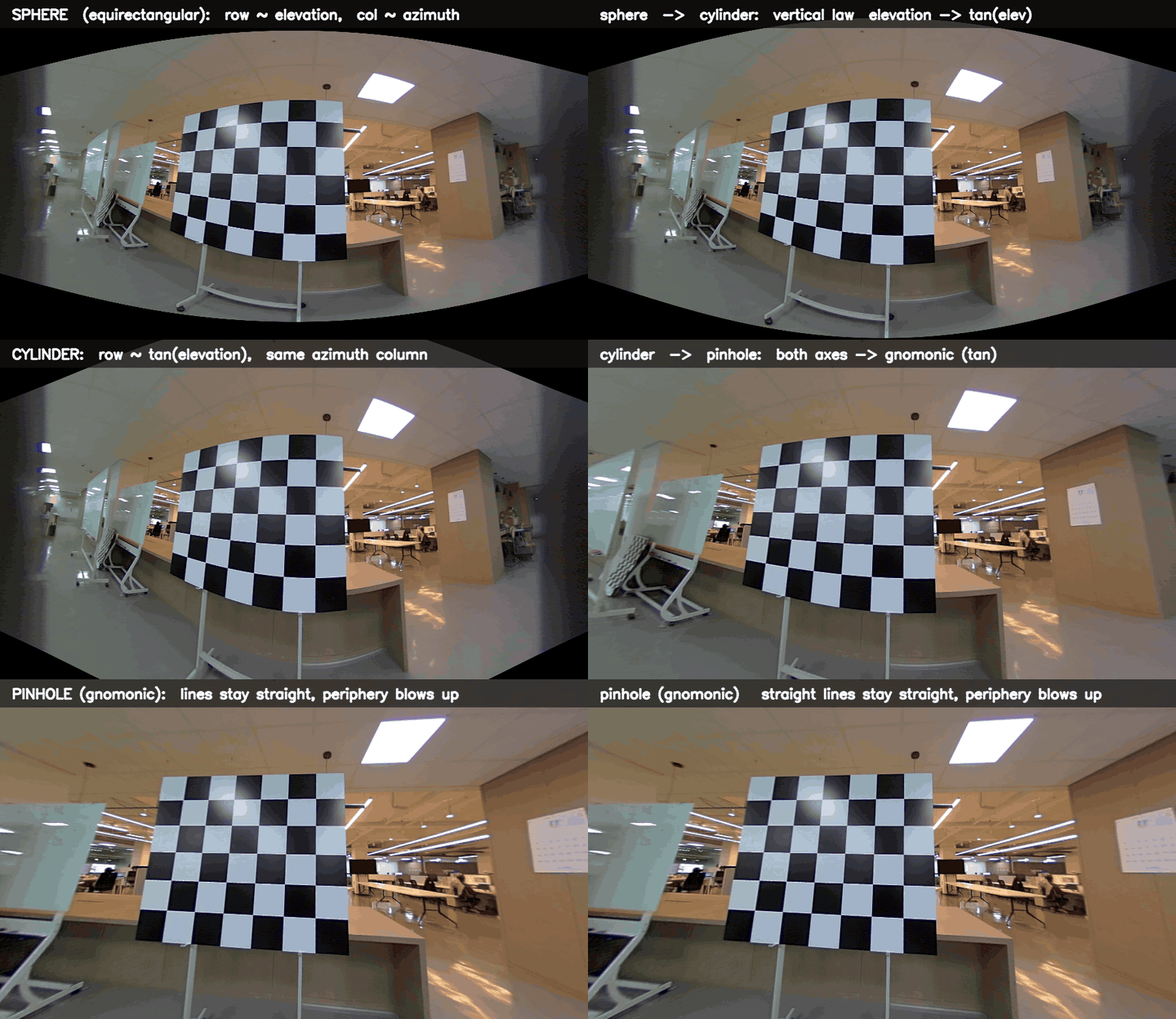
Verticals stay straight on the cylinder; the pinhole keeps lines straight but balloons the periphery and drops the polar cone to black — the >180° geometry has nowhere to land on a plane.
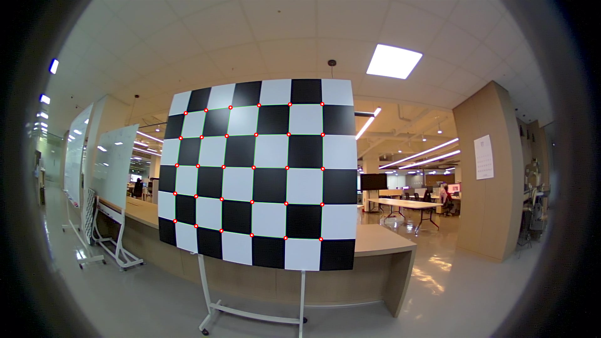
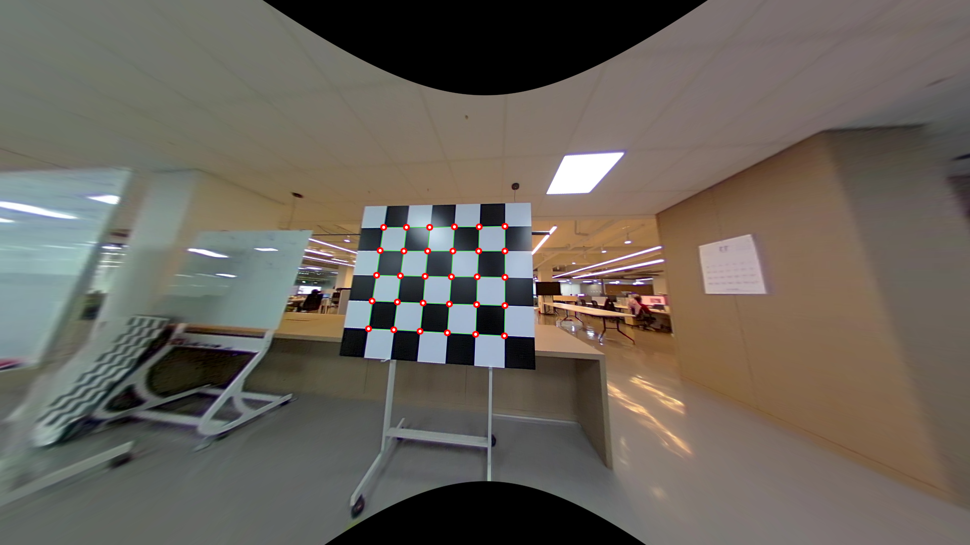
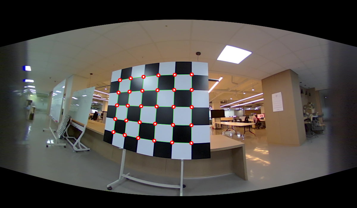
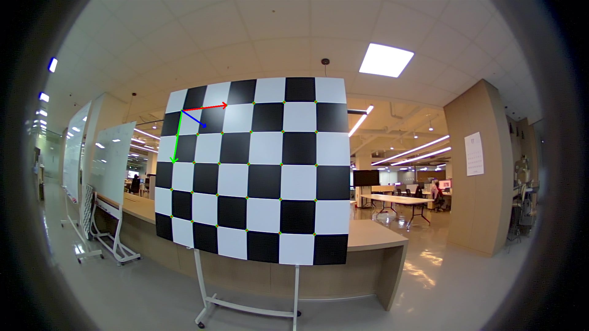
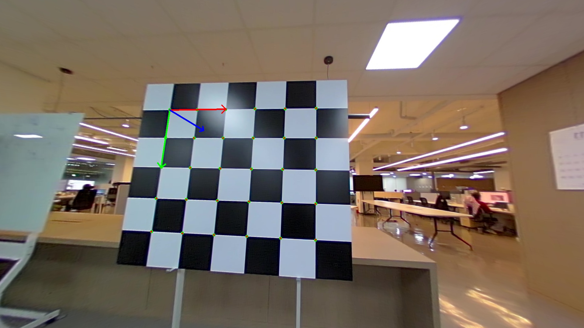
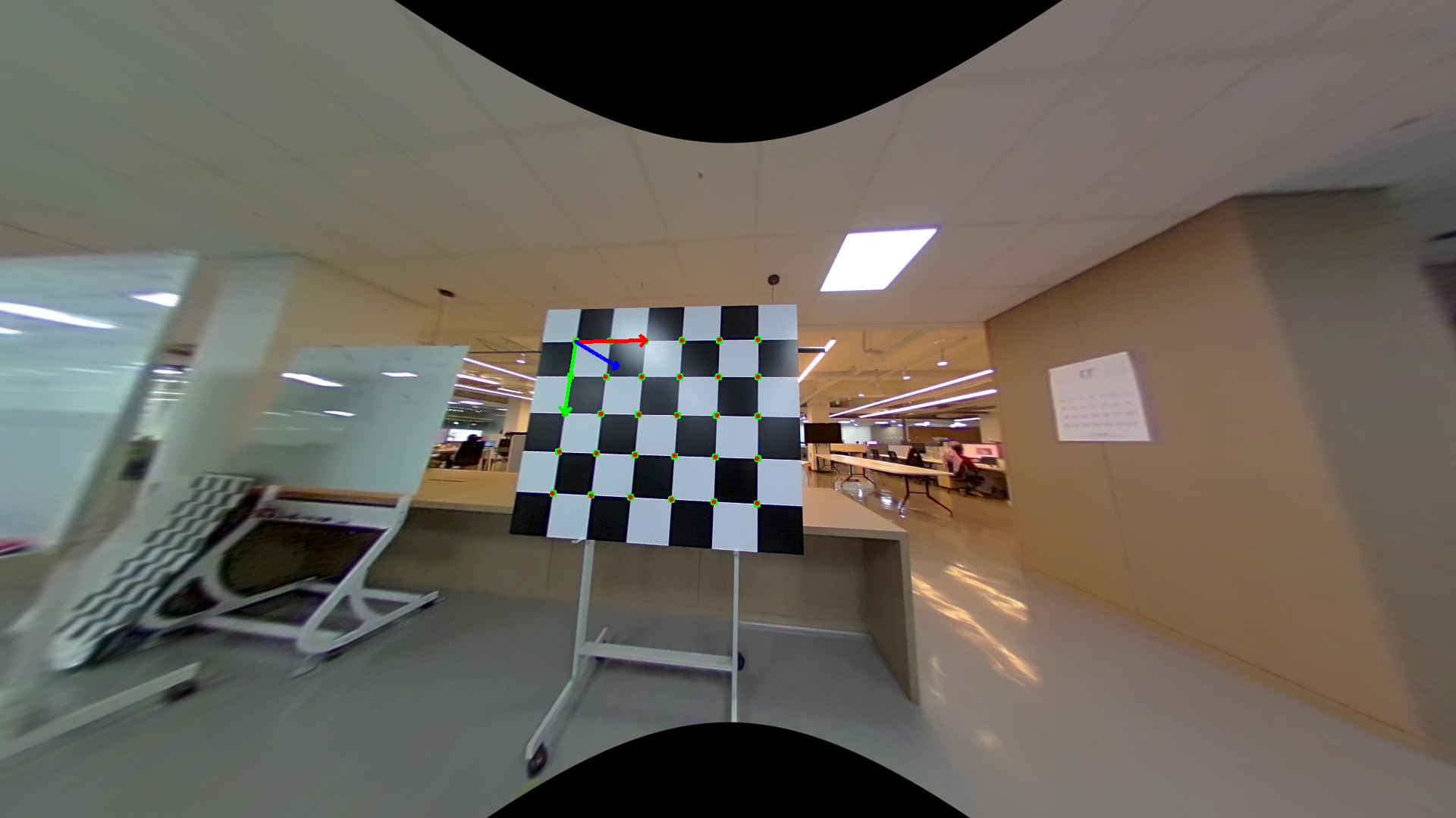
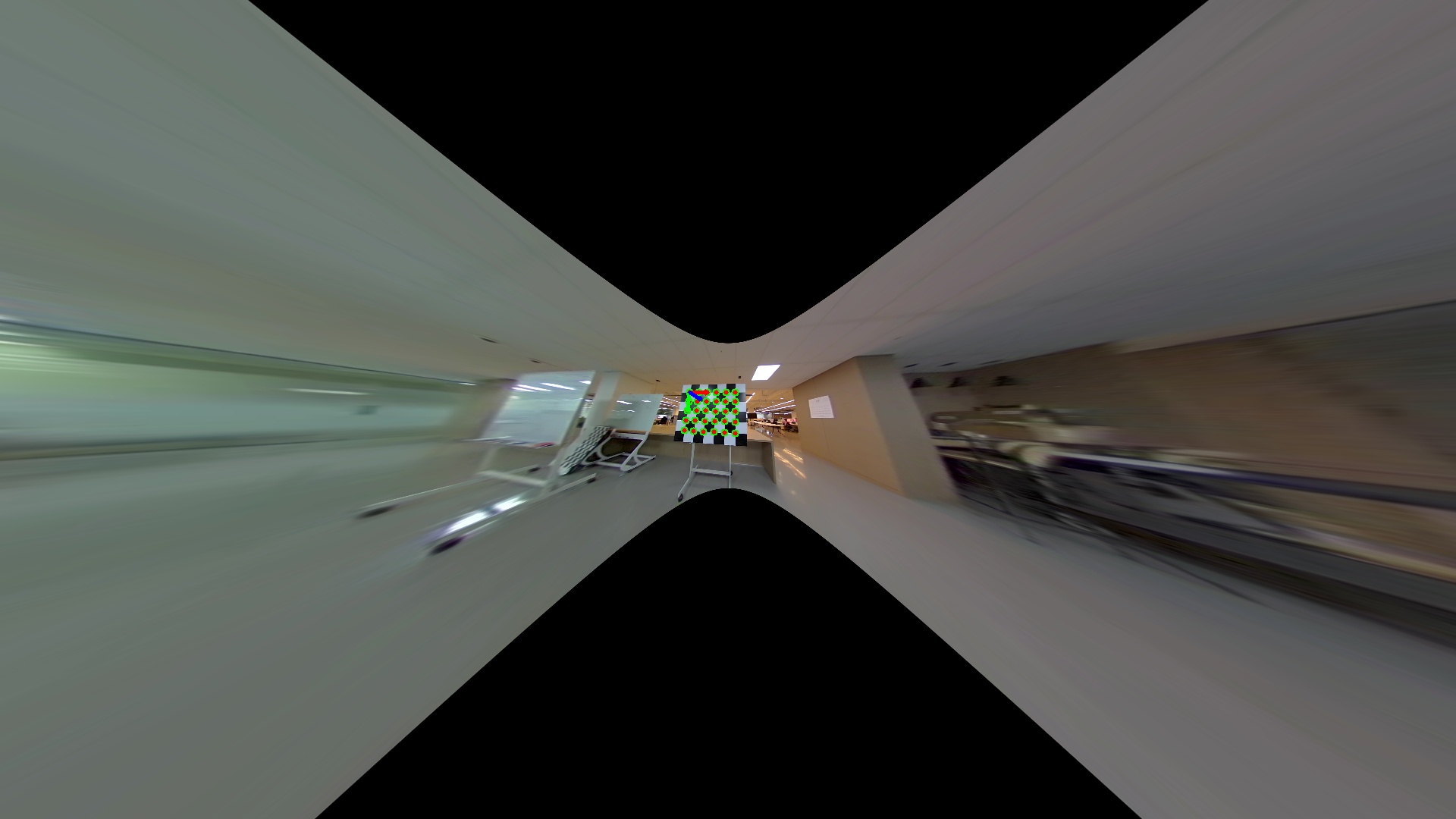
Is the conversion math actually correct? The bundled fisheye has a checkerboard with 30 known
corner pixels. We push each corner through the math — raw pixel → unproject → ray → chart pixel
— and overlay it on every representation. Every corner lands exactly on its checkerboard
intersection in all four images, and round-trips back to its raw pixel to 7e-14 px:
| Raw fisheye | Pinhole (gnomonic) |
|---|---|
 |
 |
| Sphere (equirectangular) | Cylinder |
 |
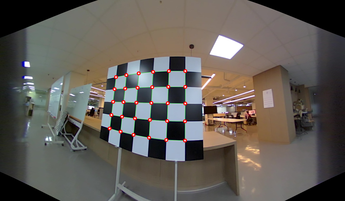 |
The board bows on the sphere, straightens on the pinhole, keeps verticals straight on the cylinder — yet no corner ever leaves the checkerboard. Full derivation, the pixel↔pixel formulas, and the per-representation round-trip table: sphere/cylinder/pinhole deep-dive (
examples/08). Every figure is generated by a checked-in script that cross-checks its frames against the library's own geometry.
Installation
Requires Python ≥ 3.10.
pip install ds-msp                 # core library
pip install "ds-msp[calib]"        # + AprilGrid detector (for the calibration capstone)
Verify:
python -c "import ds_msp; print('DS-MSP loaded:', ds_msp.__name__)"
For development (running the examples, tests, or contributing), install from source instead:
git clone https://github.com/Munna-Manoj/DS-MSP.git
cd DS-MSP
pip install -e ".[calib]"          # editable install with the detector extra
Prefer isolation?
python -m venv .venv && source .venv/bin/activate(oruv venv) first.
Quick start
A camera model is just two maps — project (3D → 2D) and unproject (2D → 3D) — plus a handful of intrinsics. They are exact inverses:
import numpy as np
from ds_msp import DoubleSphereCamera

# 6 intrinsics fully describe the lens (width/height are optional, only for image ops)
cam = DoubleSphereCamera(fx=711.57, fy=711.24, cx=949.18, cy=518.81, xi=0.183, alpha=0.809)

pts_3d = np.array([[0.0, 0.0, 1.0], [1.0, 1.0, 2.0]])   # camera-frame points (N, 3)
px,   ok = cam.project(pts_3d)     # -> (N, 2) pixels + (N,) validity mask
rays, ok = cam.unproject(px)       # -> (N, 3) unit rays  (inverse of project)
Want to see it on real data? With the [calib] extra and the TUM-VI download
(bash scripts/download_datasets.sh tumvi), calibrate a real fisheye from scratch and match the
published reference:
python examples/03_calibrate_tumvi_aprilgrid.py
Repository map
| Path | Contents |
|---|---|
ds_msp/ |
The library: core/ (contracts + Lie/LM solver + robust kernels) → pure math → models/ → services (ops/, adapt/, io/, calib/) → 3D stack (mvg/ two-view geometry, stereo/ depth, rig/ MC-Calib-compatible multi-camera calibration), plus cv.py (OpenCV-style API) and ldc.py (hardware export). |
examples/ |
Ten runnable demos on real data (01–10) — round-trip precision, the calibration capstone, robust-loss A/B, model equivalence, stereo extrinsics, the >180° validity cone, sphere/cylinder/pinhole reprojection, monocular VO, and a measurable camera-model evaluation framework. (Part II / Tier-1 demos landing — see ROADMAP.) |
docs/learn/ |
The guided curriculum (start here to learn) — Part I (calibration) + Part II (geometry & 3D). |
docs/ |
MULTI_MODEL.md (multi-model + conversion guide), ROADMAP.md, WRITING_GUIDE.md (docs style guide). |
datasets/ |
Data guide: what to download, where it goes, how to start. |
tests/ |
426 tests (contract suite, analytic-Jacobian gradient checks, calibration, two-view geometry, stereo, manifold optimization). |
The library is strictly layered (enforced in CI by import-linter): core depends on nothing, the
service layers depend only on the contract — not on concrete models or each other — and the pure-math
modules are NumPy-only.
graph TD
    services["services: ops · adapt · calib · io<br/>(work on any model via the contract)"]
    models["models: DoubleSphere · UCM · EUCM · KB · RadTan · OCam · DS⁺ · EUCM⁺<br/>(value object + pure-NumPy *_math)"]
    core["core: CameraModel contract · pinhole<br/>(dependency-free foundation)"]
    services --> core
    models -. implements .-> core
(Full diagram and design guarantees in docs/MULTI_MODEL.md.)
Learn: the guided curriculum
If you want to understand wide-FOV geometry (not just call it), the docs/learn/
track teaches it on real public data — every chapter prints a number you can verify. It runs in
two arcs: Part I — Calibration (take one camera to a published-grade calibration) and
Part II — Geometry & 3D (take that camera out into the world: two-view pose, manifold
optimization, stereo depth).
Part I — Calibration
| # | Lesson | You'll be able to… |
|---|---|---|
| 1 | Fisheye & camera models | load a published calibration, prove project/unproject invert to ~1e-14 px, rectify a real frame |
| 2 | The Double Sphere model | derive DS from first principles and read it in code |
| 🏆 | Capstone: calibrate a real camera | detect AprilGrid corners (multi-scale, periphery-robust), bundle-adjust, and match TUM-VI's published intrinsics to 0.003 % focal |
| 🔬 | Detecting every AprilGrid tag (fisheye periphery) | why an off-centre board drops to 4/36 tags, and the multi-scale + recovery fix (focal 0.7%→0.003%) |
| 🔬 | Robust losses & evaluation | handle outliers without discarding data; why median/inlier RMS beat naive RMS |
| 🔬 | Are two models the same camera? | prove DS fx≈152 and KB fx≈191 describe the same lens |
| 🔬 | Is this model right for my lens? | a measurable framework to pick a camera model — capacity, identifiability (Jacobian conditioning), parameter redundancy, cost, FOV weighting |
| 🔬 | A fair fight: EUCM⁺ vs DS⁺ vs KB | the framework applied to a real ship/retire decision — an honest good-and-bad verdict, including the hypothesis we had to retract when the data contradicted it |
| 🔬 | Sphere, cylinder & pinhole reprojection | move one fisheye between a sphere, cylinder, and pinhole image — exact pixel maps, verified to 1e-13 px |
Part II — Geometry & 3D — the wide-FOV SLAM/SfM stack. Library shipped & tested
(ds_msp/mvg/, ds_msp/core/, ds_msp/stereo/); chapters + runnable examples landing now —
see docs/learn/ and the ROADMAP. Two-view geometry on bearing vectors, manifold (SO(3)/SE(3))
pose optimization with an in-house LM solver, Schur-complement bundle adjustment, and sphere-sweep
stereo depth straight on raw fisheye.
Using the library
Full multi-model cookbook (every operation, on every model) lives in
docs/MULTI_MODEL.md. The essentials:
Create a camera
The model needs only the 6 intrinsics for projection / unprojection / PnP. width and height are
optional — required only by image-level helpers (which raise a clear error if missing).
from ds_msp import DoubleSphereCamera

# (a) math-only — no meaningless image dimensions required
cam = DoubleSphereCamera(fx=711.57, fy=711.24, cx=949.18, cy=518.81, xi=0.183, alpha=0.809)

# (b) with dimensions, for image undistortion
cam = DoubleSphereCamera(711.57, 711.24, 949.18, 518.81, 0.183, 0.809, width=1920, height=1080)

# (c) from a calibration result
cam = DoubleSphereCamera.from_json("results/calibration_params.json")

K, D = cam.K, cam.D    # 3×3 intrinsic matrix and [xi, alpha]
alphais validated to[0, 1]at construction; keepxiin[-1, 1]for the well-posed domain.
Project & unproject (+ analytic Jacobian)
import numpy as np
pts_3d = np.array([[0, 0, 1], [1, 1, 2]], dtype=np.float64)

px,   valid = cam.project(pts_3d)    # (N,2) pixels + validity (correct half-space test)
rays, valid = cam.unproject(px)      # (N,3) unit rays + validity

# Hot loops: allocation-free standalone functions + exact derivatives
from ds_msp import ds_project
from ds_msp.model import ds_project_jacobian

u, v, valid = ds_project(pts_3d, cam.fx, cam.fy, cam.cx, cam.cy, cam.xi, cam.alpha)
# J_point = d(u,v)/d(x,y,z),  J_intr = d(u,v)/d(fx,fy,cx,cy,xi,alpha)
u, v, J_point, J_intr, valid = ds_project_jacobian(
    pts_3d, cam.fx, cam.fy, cam.cx, cam.cy, cam.xi, cam.alpha)
Undistort images
Drop-in OpenCV-style API (ds_msp.cv mirrors cv2.fisheye):
import cv2, ds_msp.cv as ds_cv

img = cv2.imread("assets/test_image.jpg")
K, D = cam.K, cam.D

# balance=0.0 -> widest FOV (more scene, black borders); balance=1.0 -> tightest crop
K_new = ds_cv.estimateNewCameraMatrixForUndistortRectify(K, D, (1920, 1080), balance=0.0)
img_undist = ds_cv.undistortImage(img, K, D, Knew=K_new)
The object API is equivalent: img_undist, K_new = cam.undistort_image(img).
Robust PnP
Standard PnP assumes a pinhole model and fails on raw fisheye points. The DS solver unprojects to rays first, keeps the front-facing valid rays, then solves:
success, rvec, tvec = cam.solve_pnp(points_3d, points_2d)          # object API
success, rvec, tvec = ds_cv.solvePnP(points_3d, points_2d, cam.K, cam.D)   # OpenCV-style
Multi-model support & conversion
Calibrate in one model and translate to another without images or recalibration:
import json
from ds_msp import DoubleSphereModel, KannalaBrandtModel, convert, Undistorter, solve_pnp

ds = DoubleSphereModel.from_dict(json.load(open("results/calibration_params.json")))

kb, report = convert(ds, KannalaBrandtModel, width=1920, height=1080)   # DS -> OpenCV fisheye
print(report["rms_px"])            # sub-pixel agreement across the image

# every feature works on any model — swapping models is a one-line change
solve_pnp(kb, object_points, image_points)
img_rect, K_new = Undistorter(kb, 1920, 1080).undistort_image(img)
Supported: UCM, EUCM, Kannala-Brandt, RadTan, OCamCalib, Double Sphere, plus the two
closed-form-invertible extensions DS⁺ and EUCM⁺ (below) — all with analytic
Jacobians. You can also calibrate any model (ds_msp.calib.calibrate) and read/write Kalibr YAML
(ds_msp.io). Conversion design follows
Fisheye-Calib-Adapter (see Credits).
DS⁺ / EUCM⁺ — closed-form models for lenses that defeat Double Sphere
Two spherical models with extra invertible distortion stages for lenses whose radial curve falls outside the rigid 2-DOF Double-Sphere manifold (see the FOV note below):
- DS⁺ = UCM core + 2-term Fitzgibbon division (θ³, θ⁵) + 2-axis Scheimpflug tilt. 9 params. Closed-form inverse (one cube root). Most accurate and the most robust to seed; our default when accuracy matters most.
- EUCM⁺ = EUCM core (
α, β) + 1-term division + 2-axis tilt. 9 params. Truly closed-form, square-root-only inverse — no cube root, no Newton iteration — so it round-trips to ~1e-9° and unprojects in DS-class cycles.
from ds_msp.models import DSPlusModel, EUCMPlusModel          # or model_class("dsplus")/("eucm+")
cam = EUCMPlusModel.from_dict(json.load(open("eucm_plus_parameters.json")))
Both register by name (dsplus, eucmplus, aliases ds+/eucm+), satisfy the full CameraModel
contract (project / unproject / analytic Jacobian / convert / Kalibr+MC-Calib I/O), and reduce
exactly to their parent (DS⁺→UCM, EUCM⁺→EUCM) when the extra DOF are zero.
Choosing a model by FOV (from experience)
A practical finding from calibrating real lenses across the range: the spherical family
(UCM / EUCM / Double Sphere) can quietly collapse on smaller wide-angle lenses (~120–140°) yet
fit cleanly on very wide ones (170–195°). On a ~140° checkerboard lens here, Double Sphere drove
ξ→0 (one sphere goes dead) and floored at ~2–3 px; on 170° and 195° lenses the same model dropped
to the detection limit (~0.08–0.6 px) with no trouble. The reason is geometric, not a bug: a
moderate-FOV lens whose radial curve needs a θ⁵ term plus a little decentering sits outside DS's
2-DOF curve, while a true ultra-wide lens bends enough that the two-sphere shape matches it. So
"more distortion" is actually easier for the sphere models — counterintuitive but consistent.
What we reach for, by FOV band (✅ recommended · ⚠️ works with care · ❌ avoid):
| Model | ~120–140° (small wide) | 170–195° (ultra wide) | Notes from use |
|---|---|---|---|
| RadTan (OpenCV pinhole) | ⚠️ | ❌ | Fine for mild distortion; the X/Z projection blows up approaching 180° — not a fisheye model. |
| KB (OpenCV fisheye) | ✅ | ✅ | The dependable conventional baseline at every band (~0.35 px @140°, detection-limited beyond). Iterative (Newton) unproject. |
| UCM / EUCM / Double Sphere | ❌ (collapse risk) | ✅ | Closed-form & cheap, but can degenerate at ~140° (ξ/α collapse). Excellent once the lens is genuinely ultra-wide. |
| DS⁺ | ✅ (best accuracy) | ✅ | Restores the missing DOF; most accurate (~0.21 px @140°) and converges from a plain seed at any FOV. Inverse uses one cube root. |
| EUCM⁺ | ✅ | ✅ | Truly sqrt-only closed form; ~0.29 px @140°. At ~140° seed it multi-start; at 170–195° a single seed suffices. |
Rule of thumb: ultra-wide (≥170°) → start with Double Sphere (cheapest closed form that fits). Smaller wide-angle (~120–150°) → if DS/EUCM collapse, move to KB (conventional) or, for a closed-form inverse, DS⁺ / EUCM⁺. Always confirm with the median reprojection error rather than trusting the model class.
Numbers above are from this repo's datasets (a ~140° checkerboard lens, a 170°
annslens, and a 195° TUM-VI lens); treat them as directional guidance, not guarantees for your optics.
Hardware LDC export (TI Jacinto)
Generate a displacement-mesh LUT for the on-chip Lens Distortion Correction engine (J7 / TDA4):
from ds_msp.ldc import TI_LDC_MeshGenerator

gen = TI_LDC_MeshGenerator(cam)                  # cam built with width/height
res = gen.generate_mesh_and_intrinsics(1920, 1080, downsample_factor=4, balance=0.5)
mesh_lut, K_new = res["mesh_lut"], res["K_new"]  # int16 Q3 displacements + rectified intrinsics
Best practice: use the LDC image for the picture, but undistort keypoints with the closed-form
cam.undistort_points(pts, K_new)at the samebalance. The mesh point-inverse is exact at the center but diverges toward the periphery; sharingK_newkeeps the two consistent to ~0.1 px.
Calibration
Calibrate the intrinsics of any model from your own images: detect corners with OpenCV, hand the
3D↔2D correspondences to the generic backend, done. ds_msp.calib.calibrate is model-agnostic —
the same call fits DS, UCM, EUCM, KB, RadTan, OCam, DS⁺ or EUCM⁺; only the seed class changes. It
runs a manifold Levenberg–Marquardt solve with analytic Jacobians and an optional robust loss,
so a few mis-detected corners down-weight instead of dragging the fit.
From a checkerboard with OpenCV (the common case)
import cv2, glob, numpy as np
from ds_msp.calib import calibrate
from ds_msp.models import KannalaBrandtModel       # swap for DoubleSphereModel, EUCMModel, DSPlusModel, …

# board geometry: the inner-corner grid of your printed checkerboard, in metres
COLS, ROWS, SQUARE = 9, 6, 0.025
objp = np.zeros((ROWS * COLS, 3), np.float64)
objp[:, :2] = np.mgrid[0:COLS, 0:ROWS].T.reshape(-1, 2) * SQUARE

# 1. detect corners with OpenCV in every calibration frame
X_world, keypoints, visibility, shape = [], [], [], None
for path in sorted(glob.glob("calib_images/*.png")):
    gray = cv2.imread(path, cv2.IMREAD_GRAYSCALE)
    shape = gray.shape
    found, corners = cv2.findChessboardCornersSB(gray, (COLS, ROWS), cv2.CALIB_CB_EXHAUSTIVE)
    if not found:
        continue                                    # SB detector is sub-pixel by design
    X_world.append(objp.copy())
    keypoints.append(corners.reshape(-1, 2).astype(np.float64))
    visibility.append(np.ones(len(objp), bool))     # all corners seen (partial boards are fine too)

# 2. calibrate ANY model from a generic seed (cx,cy = image centre; a rough focal is fine —
#    per-view poses are re-seeded internally). loss="huber" down-weights stray corners.
h, w = shape
seed = KannalaBrandtModel(fx=0.5 * w, fy=0.5 * w, cx=0.5 * w, cy=0.5 * h)
result = calibrate(seed, X_world, keypoints, visibility, loss="huber", f_scale=1.0)

print(result["model"])                              # calibrated intrinsics
print("reprojection RMS:", result["rms_px"], "px")  # quality check
result["model"].to_dict()                           # JSON-ready (or convert(...) to another model)
That's the whole loop — OpenCV finds the corners, the backend fits the model. To try a different
model, change only the seed class (see Choosing a model by FOV
for which fits your lens); to switch the calibrated result to another model afterwards, use
convert — no re-detection needed.
From an AprilGrid (robust across the fisheye periphery)
For wide fisheye lenses an AprilGrid keeps corners detectable out to the rim. This is what the capstone uses on real TUM-VI footage:
import glob
from ds_msp.calib import calibrate, AprilGridTarget, detect_aprilgrid
from ds_msp.models import KannalaBrandtModel

# 1. detect AprilGrid corners in your calibration frames
frames = sorted(glob.glob("datasets/tumvi/dataset-calib-cam1_512_16/mav0/cam0/data/*.png"))
detections = detect_aprilgrid(frames, family="t36h11")

# 2. turn tag detections into 3D<->2D correspondences (board geometry: 6x6, 88 mm, spacing 0.3)
target = AprilGridTarget(tag_rows=6, tag_cols=6, tag_size=0.088, tag_spacing=0.3)
X_world, keypoints, visibility = target.build_correspondences(detections)

# 3. bundle-adjust from a generic seed (analytic Jacobian + robust Cauchy loss)
seed = KannalaBrandtModel(fx=180, fy=180, cx=256, cy=256)
result = calibrate(seed, X_world, keypoints, visibility, loss="cauchy", f_scale=0.5)
print(result["rms_px"])      # sub-pixel; the capstone reports 0.08 px median, matching the published calibration
See the full walk-through in the calibration capstone.
The bundled Double Sphere script
A ready-to-run script calibrates Double Sphere from COCO-style checkerboard annotations:
python calibrate.py        # reads anns.json -> writes results/calibration_params.json
python validate.py         # visual reprojection check -> results/visualizations/
On the bundled data this converges to fx≈711.6, fy≈711.2, cx≈949.2, cy≈518.8, xi≈0.183, alpha≈0.809
at 0.64 px RMS.
Parameter domain (important). The optimizer constrains distortion to the well-posed Double Sphere range
α ∈ [0, 1],ξ ∈ [-1, 1](matching basalt/Kalibr). Outside it the model becomes non-injective (projection folds back, so unprojection can't invert it); real fisheye lenses sit roughly inξ ∈ [-0.2, 0.6].
Multi-camera rig calibration (MC-Calib-compatible)
Status — preview, landing in 0.8.0. The rig pipeline is implemented and tested on synthetic and real multi-camera data, but is not yet part of the
pip install ds-mspwheel: run it from a source checkout viascripts/calibrate_rig.py. Governed underFR-RIG-*in the project's engineering process.
Beyond single-camera intrinsics, DS-MSP ships ds_msp.rig — the N-camera analogue of
MC-Calib. It calibrates the extrinsics (where every
camera sits relative to the others) plus per-camera intrinsics from a folder of ChArUco images,
driven by a single MC-Calib-style calib_param.yml. It is drop-in with MC-Calib — the same
config schema and the same output files — with one extension: a different camera model per camera,
chosen from any of DS-MSP's eight models (so one bench can mix kb fisheye, radtan pinhole, and
dsplus).
# from a source checkout (the rig is not in the pip wheel yet)
python scripts/calibrate_rig.py --init-config calib_param.yml   # write a starter config
# edit it (cameras, board geometry, image folder, models), then:
python scripts/calibrate_rig.py --config calib_param.yml
Faithful to MC-Calib's workflow: ChArUco detection → multi-board fused-object reconstruction (the
calibrate3DObjects analogue) → camera-group extrinsics init → staged global bundle adjustment →
MC-Calib-format results (calibrated_cameras_data.yml, calibrated_objects_data.yml, …). With two
DS-MSP additions:
- Per-camera initial intrinsics — provide a
camera_parametersYAML; the rig loads it, checks the stated model matches your config, then holds it fixed (fix_intrinsic=1, extrinsics-only) or refines it. If the chosen model differs, it carries the same lens into that model viaconvert()and warns — so the run proceeds either way. - Detect-once, calibrate-many — detected corners are saved to
detected_keypoints_data.ymland reused viakeypoints_path, so you can re-calibrate with different models / options in seconds instead of re-detecting.
On a real 8-camera rig (mixed fisheye + pinhole), the pipeline matches or beats a from-scratch baseline and is robust to how intrinsics are supplied — from-scratch, provided-and-refined, and provided-and-held-fixed all converge to the same extrinsics (≤ 0.05° / 2 mm) and reprojection error.
Developers — want to use or extend it?
- Use it: the full guide — data layout, folder/image naming, every config field, extrinsics-only
mode, and the keypoints-reuse workflow — is in
docs/RIG_CALIBRATION_GUIDE.md. Starter configs:configs/calib_param.template.yml,configs/calib_param.keypoints.template.yml,configs/camera_intrinsics.template.yml. - Extend it: the contributor recipe (requirements → tier rules → MC-Calib parity → tests → docs) is the rig playbook.
Deep dive: FOV, validity & undistortion
A common question: "Why are pixels missing from my undistorted image, even when I try to keep the whole image?"
Undistortion modes
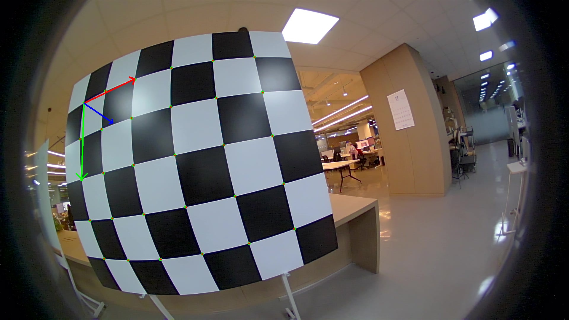
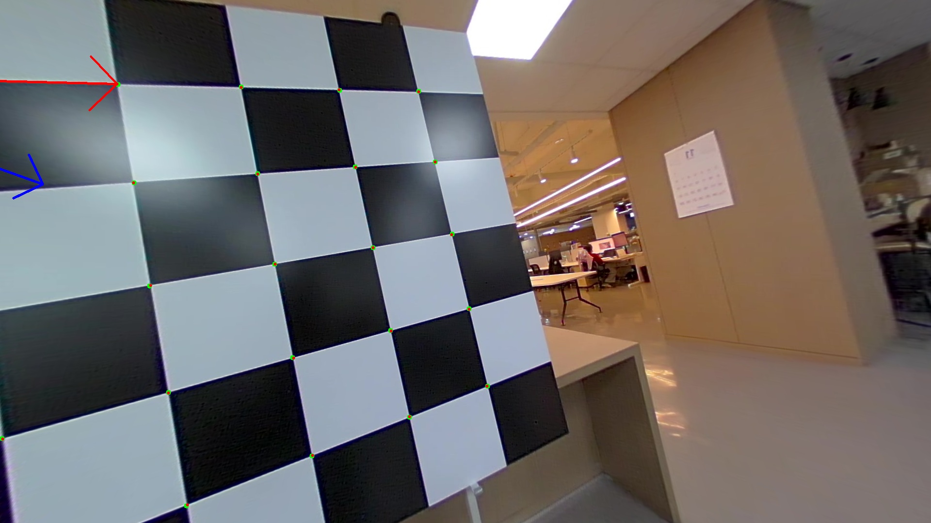
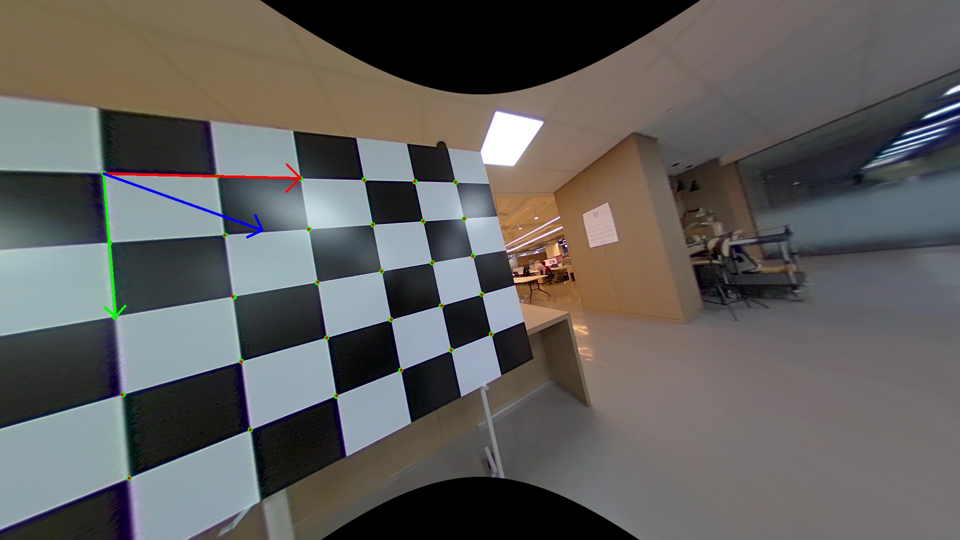
Verified on real data (assets/test_image.jpg, assets/test_image_96.jpg):
| Distorted | Undistorted (crop) | Undistorted (whole) | Undistorted (zoom) |
|---|---|---|---|
 |
 |
 |
 |
 |
 |
 |
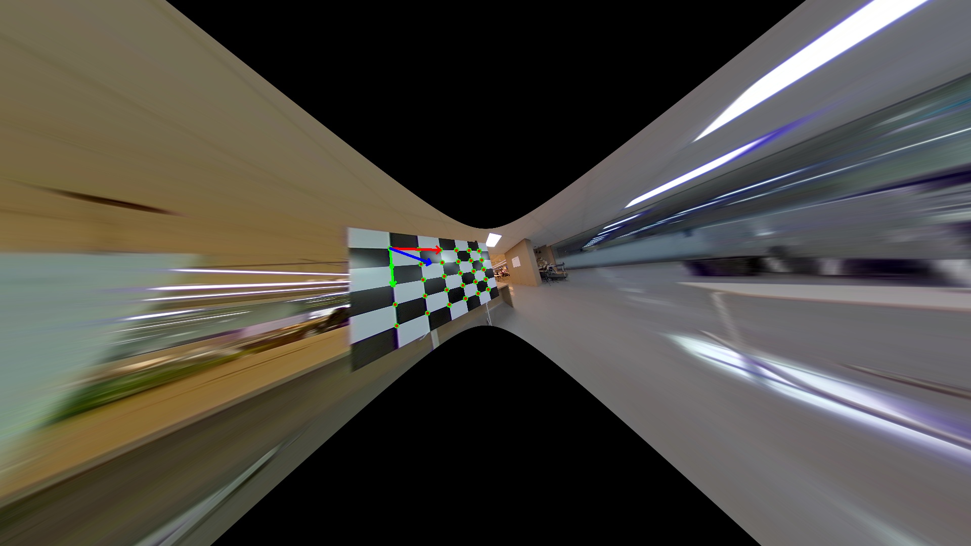 |
- Crop (
balance=1.0) — keeps only center-valid pixels: no black borders, less FOV. - Whole (
balance=0.0) — keeps all pixels that map to the plane: full content, black borders. - Zoom (reduced focal) — captures even more wide-angle content, shrinking the center.
Projection validity — the correct condition
The Double Sphere projection π(x) is not valid for all 3D points. The exact projectability test
(Usenko et al. 2018, Eq. 43–45), implemented in ds_project, is the half-space condition:
$$z > -w_2, d_1, \qquad d_1 = \sqrt{x^2 + y^2 + z^2}$$
with the two helper terms
$$ w_1 = \begin{cases} \dfrac{\alpha}{1-\alpha} & \text{if } \alpha \le 0.5 \ \dfrac{1-\alpha}{\alpha} & \text{if } \alpha > 0.5 \end{cases} $$
$$ w_2 = \frac{w_1 + \xi}{\sqrt{2, w_1 \xi + \xi^2 + 1}} $$
This admits points with z ≤ 0 (rays beyond 90°), which is exactly why the model supports a
> 180° FOV. A naive z > 0 test — a common implementation mistake — rejects those rays and
silently caps the FOV below 180°; this library does not make that mistake.
Forward / inverse equations (for reference)
$$d_2 = \sqrt{x^2 + y^2 + (\xi d_1 + z)^2}, \qquad \begin{bmatrix} u \ v \end{bmatrix} = \begin{bmatrix} f_x, x / \big(\alpha d_2 + (1-\alpha)(\xi d_1 + z)\big) + c_x \ f_y, y / \big(\alpha d_2 + (1-\alpha)(\xi d_1 + z)\big) + c_y \end{bmatrix}$$
Unprojection is closed-form; with $m_x=(u-c_x)/f_x$, $m_y=(v-c_y)/f_y$, $r^2=m_x^2+m_y^2$ it is valid for all $r^2$ when $\alpha \le 0.5$, and for $r^2 \le 1/(2\alpha-1)$ when $\alpha > 0.5$.
Valid parameter domain: $\alpha \in [0, 1]$, $\xi \in [-1, 1]$.
The FOV zones
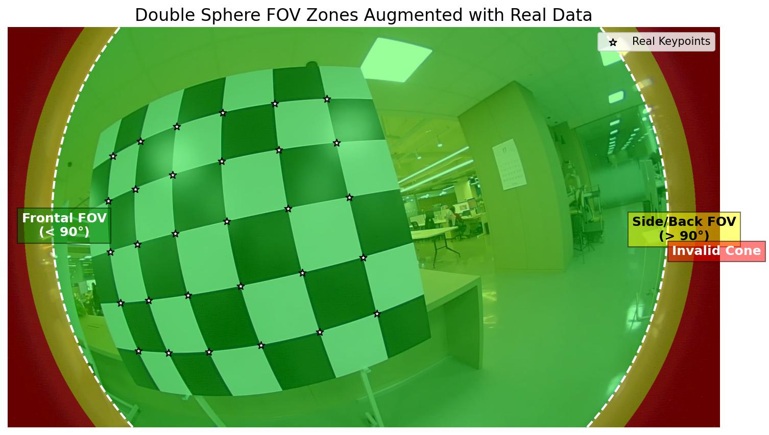
- Green (frontal,
θ < 90°) — safe for standard pinhole projection. - Yellow (side/back,
90° ≤ θ < θ_limit) — valid in DS, but impossible to project into a single pinhole image (Z ≤ 0): a pinhole plane is infinite at 90°, so these pixels have nowhere to go. - Red (
θ ≥ θ_limit) — mathematically invalid in DS. - White stars — real keypoints, all safely inside the valid regions.
This is why undistortion can't keep a full > 180° FOV: those wide-angle pixels are not lost to a bug, they are geometrically un-pinhole-able. (Reference: projection-failed region analysis.)
Accuracy & verification
Correctness is asserted with numbers, not screenshots (tests/, verify_real_samples.py):
| Check | Result |
|---|---|
Inverse projection K⁻¹ (all undistortion modes) |
mean error < 0.00003 px ✅ |
| 3D reconstruction of checkerboard corners | mean position error 1.168 mm; recovered square 20.01 cm (target 20.00) ✅ |
PnP + reprojection RMS (real test_image / _96) |
0.43 px / 0.85 px |
Undistort: object API vs cv.py wrapper |
identical |
| KB / RadTan vs OpenCV | match to ~1e-13 |
Conclusion: the undistorted images are geometrically accurate pinhole projections suitable for
precise 3D vision. Reproduce locally with bash verify_all.sh or pytest; for the accuracy/speed
numbers above, run python benchmarks/benchmark.py (e.g. KB vs cv2.fisheye to
~1e-13 px; analytic Jacobian ~28× faster per LM iteration than finite differences).
FAQ
My undistorted image has black borders?
Normal for fisheye — a pinhole view can't capture the full > 180° FOV. Tune balance in
estimateNewCameraMatrixForUndistortRectify to trade border vs FOV.
PnP fails or gives bad results?
Use cam.solve_pnp(...) (or ds_msp.cv.solvePnP), not cv2.solvePnP — the latter assumes pinhole and
fails on raw fisheye points. You need ≥ 4 points that are in front of the camera after unprojection.
What ranges are valid for xi and alpha?
alpha ∈ [0, 1] (enforced at construction) and xi ∈ [-1, 1]. Beyond that the model is non-injective;
the calibrator constrains to this domain automatically. Real lenses sit in xi ∈ [-0.2, 0.6].
Do I have to pass width and height?
No — only for image-level operations (undistortion maps / compute_K_new). Projection, unprojection,
Jacobians, and PnP need just the 6 intrinsics.
How do I use this with ROS?
Wrap ds_msp.cv.undistortImage in a node: subscribe to image_raw, undistort, publish image_rect.
Roadmap
DS-MSP is actively growing from a camera library into a small perception toolkit (multi-camera &
camera-IMU calibration, visual odometry on public benchmarks, a C++/Ceres core, inference-only learned
3D). See docs/ROADMAP.md for the build order and design rules.
Credits
This project builds on excellent open-source work and research.
Model conversion (the multi-model adapter)
- Fisheye-Calib-Adapter — Sangjun Lee, "Fisheye-Calib-Adapter: An Easy Tool for Fisheye Camera Model Conversion", arXiv:2407.12405 (2024) · github.com/eowjd0512/fisheye-calib-adapter. Our conversion design (sample → unproject with the source → linear-seed → nonlinear refine on pixel reprojection error, per-model analytic Jacobians) and the set of supported models follow this work.
Camera models
- Double Sphere — V. Usenko, N. Demmel, D. Cremers, "The Double Sphere Camera Model", 3DV 2018, arXiv:1807.08957. Reference: basalt-headers (half-space validity condition & analytic Jacobians follow it).
- Kannala-Brandt (equidistant) — J. Kannala, S. Brandt, 2006; cross-checked vs OpenCV
cv2.fisheye. - Radial-Tangential (Brown-Conrady) — D. C. Brown, 1966; cross-checked vs OpenCV
cv2.projectPoints. - OCamCalib — D. Scaramuzza et al. · EUCM — Khomutenko, Garcia, Martinet, 2016 · UCM — Geyer & Daniilidis / Mei & Rives.
Calibration ecosystem & tooling
- MC-Calib — F. Rameau, J. Park, O. Bailo, I. S. Kweon, "MC-Calib: A generic and robust
calibration toolbox for multiple cameras", Computer Vision and Image Understanding (CVIU), 2022 ·
github.com/rameau-fr/MC-Calib. DS-MSP's multi-camera rig
pipeline (
ds_msp.rig) is a Python re-implementation that follows MC-Calib's design: itscalib_param.ymlconfig schema, its result-file format (calibrated_cameras_data.yml, …), and its workflow (ChArUco multi-board object reconstruction, camera groups, staged bundle adjustment). Files are interoperable in both directions; full credit for the original toolbox and format goes to the MC-Calib authors. - Kalibr — P. Furgale et al., github.com/ethz-asl/kalibr
(DS & EUCM contributed by V. Usenko). We follow Kalibr's
camchainYAML format for interop. - dscamera — Python DS utilities.
- Double Sphere explanation & projection-failed region — clear write-ups.
This codebase
- Muhammadjon Boboev — original Python Double Sphere intrinsics calibration this project grew from.
License
Dual-licensed (see LICENSING.md):
- The generic library is MIT — free for any use, including commercial (standard KB/DS/UCM/EUCM/RadTan models, geometry, I/O, detection, evaluation).
- The project's core contribution is PolyForm Noncommercial 1.0.0 —
the DS+/EUCM+ models (
ds_msp/models/{dsplus,eucmplus}*.py) and the robust from-scratch calibration/conversion engine (ds_msp/geometry/resection.py,ds_msp/calib/bundle.py,ds_msp/adapt/convert.py) — free for research, academic, personal and other noncommercial use with attribution to Munna-Manoj; commercial use requires a separate license from the author.
SPDX: MIT AND LicenseRef-PolyForm-Noncommercial-1.0.0. Please cite via CITATION.cff.
Project details
Verified details
These details have been verified by PyPIProject links
GitHub Statistics
Maintainers
Release history Release notifications | RSS feed


Download files
Download the file for your platform. If you're not sure which to choose, learn more about installing packages.
Source Distribution
Built Distribution
Filter files by name, interpreter, ABI, and platform.
If you're not sure about the file name format, learn more about wheel file names.
Copy a direct link to the current filters
File details
Details for the file ds_msp-0.8.0.tar.gz.
File metadata
- Download URL: ds_msp-0.8.0.tar.gz
- Upload date:
- Size: 166.9 kB
- Tags: Source
- Uploaded using Trusted Publishing? Yes
- Uploaded via: twine/6.1.0 CPython/3.13.12
File hashes
| Algorithm | Hash digest | |
|---|---|---|
| SHA256 |
95e0acf2035aa8940bd377f56f007c9b133b4ae87247b2609353706c3b2e7a07
|
|
| MD5 |
aefb62be707ab48e8ded9f399c61f27f
|
|
| BLAKE2b-256 |
013507bc4e8a5197cc9c925c37fd2384455a7dcada0dfecc8196cbada26ffd8d
|
Provenance
The following attestation bundles were made for ds_msp-0.8.0.tar.gz:
Publisher:
release.yml on Munna-Manoj/DS-MSP
-
Statement:
-
Statement type:
https://in-toto.io/Statement/v1 -
Predicate type:
https://docs.pypi.org/attestations/publish/v1 -
Subject name:
ds_msp-0.8.0.tar.gz -
Subject digest:
95e0acf2035aa8940bd377f56f007c9b133b4ae87247b2609353706c3b2e7a07 - Sigstore transparency entry: 2015169870
- Sigstore integration time:
-
Permalink:
Munna-Manoj/DS-MSP@4afeb2a6072ac855e9a37dc387dfa953ca9b6b73 -
Branch / Tag:
refs/heads/main - Owner: https://github.com/Munna-Manoj
-
Access:
public
-
Token Issuer:
https://token.actions.githubusercontent.com -
Runner Environment:
github-hosted -
Publication workflow:
release.yml@4afeb2a6072ac855e9a37dc387dfa953ca9b6b73 -
Trigger Event:
push
-
Statement type:
File details
Details for the file ds_msp-0.8.0-py3-none-any.whl.
File metadata
- Download URL: ds_msp-0.8.0-py3-none-any.whl
- Upload date:
- Size: 168.6 kB
- Tags: Python 3
- Uploaded using Trusted Publishing? Yes
- Uploaded via: twine/6.1.0 CPython/3.13.12
File hashes
| Algorithm | Hash digest | |
|---|---|---|
| SHA256 |
2e3f5fe4085df3f35427e675ac97fd1bbac6319572a6030822861877236f195c
|
|
| MD5 |
2f4dceaeaf121f764a33a23aa76cf62c
|
|
| BLAKE2b-256 |
afecedf10dea27dafd2163e0d73e20350b2175aaa52c6939f50957dbecd5e5cd
|
Provenance
The following attestation bundles were made for ds_msp-0.8.0-py3-none-any.whl:
Publisher:
release.yml on Munna-Manoj/DS-MSP
-
Statement:
-
Statement type:
https://in-toto.io/Statement/v1 -
Predicate type:
https://docs.pypi.org/attestations/publish/v1 -
Subject name:
ds_msp-0.8.0-py3-none-any.whl -
Subject digest:
2e3f5fe4085df3f35427e675ac97fd1bbac6319572a6030822861877236f195c - Sigstore transparency entry: 2015169950
- Sigstore integration time:
-
Permalink:
Munna-Manoj/DS-MSP@4afeb2a6072ac855e9a37dc387dfa953ca9b6b73 -
Branch / Tag:
refs/heads/main - Owner: https://github.com/Munna-Manoj
-
Access:
public
-
Token Issuer:
https://token.actions.githubusercontent.com -
Runner Environment:
github-hosted -
Publication workflow:
release.yml@4afeb2a6072ac855e9a37dc387dfa953ca9b6b73 -
Trigger Event:
push
-
Statement type:






