
Easy-EO

| Install |     |
| Build & quality |      |
| Security |   |
| Project |    |
Easy-EO is a lightweight, extensible Python library for raster-based Earth Observation (EO) analysis. It covers searching and loading imagery, cloud masking, band algebra and spectral indices, time series and visualization, and each step is a few readable lines of Python.
From satellite archive to NDVI map
import eeo

results = eeo.stac_search(
    collection="sentinel-2-l2a",
    bbox=(11.0, 46.5, 11.2, 46.7),        # area of interest, WGS 84 lon/lat
    datetime="2023-06-01/2023-08-31",
    cloud_cover=20,
    limit=1,
)
scene = results[0].load(assets=["B04", "B08"])   # reads only the area of interest
ndvi = scene.ndvi(red="B04", nir="B08")
ndvi.plot_raster()
That is the whole workflow: no scene downloads and no GDAL wrangling. The search
queries Microsoft Planetary Computer
by default, and any other STAC catalog works through catalog="<catalog URL>".
The load streams only the window covering your bounding box over HTTP, which
here is 14 MB out of a 240 MB Sentinel-2 tile and takes a few seconds.
stac_search needs the STAC extra: pip install "easy-eo[stac]", or the
conda equivalent. To start offline instead, jump to the
hosted sample dataset, which needs no network after the first
call.
Features
| What you get | Guide | |
|---|---|---|
| Catalog search | stac_search() over any STAC catalog, by bounding box or by a polygon; loading reads only your area of interest over HTTP; deduplicate() drops reprocessed copies of the same acquisition |
Satellite data |
| Downloaded products | load_sentinel2() and load_landsat() read a Sentinel-2 L2A .SAFE or a Landsat Collection 2 product as you downloaded it, still zipped or tarred, with bands chosen by name and the acquisition time recorded |
Downloaded scenes |
| Cloud masking | mask_clouds() sets cloud, cloud shadow and cirrus to nodata from the Sentinel-2 scene classification or the Landsat QA_PIXEL band, including medium-confidence cloud; clear_fraction() reports how much of a scene is left |
Masking clouds |
| Time series | time_series() builds a series from a search, a folder of GeoTIFFs or scenes you loaded; map() applies any operation to every date; median/mean/min/max, cloud-free composite(), monthly or weekly resample_time(); extract_at() returns a pixel's trajectory as a pandas DataFrame |
Time series |
| Spectral indices | ndvi, ndwi, ndmi, ndbi, evi, savi, plus normalized_difference for anything else, all chainable and float32 |
Spectral indices |
| Band algebra | add, subtract, multiply, divide, power, sqrt, log, absolute, and the matching operators |
Operations |
| Preprocessing | Clip to a bounding box or a vector, resample, reproject, mosaic, stack, normalize (min-max, percentile, z-score) | Preprocessing |
| Large rasters | Algebra, indices and normalization run a block at a time; apply_blockwise() streams a computation of your own to disk; load_raster(path, chunks=...) opens a raster lazily with dask, including a COG over HTTP |
Large rasters |
| Named bands and metadata | Address any band as "red" or "nir" wherever a 1-based index works; names survive a GeoTIFF round-trip; a timestamp and free-form attrs follow the data through every operation; describe() summarises a raster without reading its pixels |
Naming bands · The dataset |
| Statistics | Per-band min/max/mean/percentile with their pixel locations, and value extraction at a coordinate | Statistical locations |
| Visualization | Single bands, RGB composites, histograms, map-plus-histogram views, and for a series a trajectory plot and a filmstrip of dates, all read at display resolution | Visualization |
| Predictable nodata and dtype | One written-down contract every operation follows: mask before compute, nodata stays contagious, fractional results are float32 | Nodata and dtype |
| Ecosystem interop | to_xarray() / from_xarray() in both directions, and to_xarray() on a whole series; NumPy, Rasterio and xarray backends behind one interface |
xarray interop · Backends |
| Typed and tested | Ships py.typed, 2,800+ tests, 99% coverage, checked on Python 3.10-3.14 across Linux, macOS and Windows |
Contributing |
Before and after
One ordinary task: clip a 4-band scene to an area of interest held in a vector file, compute NDVI, and save it as a GeoTIFF. Both versions below run as written, against the same hosted sample dataset (a 1024x1024 Sentinel-2 subset and a boundary polygon), so you can paste either one and watch it work.
Here it is in raw Rasterio, GeoPandas and NumPy, with Easy-EO not installed at all:
import geopandas as gpd
import numpy as np
import rasterio
from rasterio.mask import mask

BASE = "https://github.com/Tommy-Burns/easy-eo/releases/download/sample-data-v1/"

with rasterio.open(BASE + "sentinel2_small_cog.tif") as src:
    aoi = gpd.read_file(BASE + "roi.gpkg").to_crs(src.crs)
    clipped, transform = mask(src, aoi.geometry.values, crop=True)
    bands = {name: i for i, name in enumerate(src.descriptions)}
    nodata = src.nodata
    profile = src.profile

red = clipped[bands["red"]].astype("float32")
nir = clipped[bands["nir"]].astype("float32")

valid = (red != nodata) & (nir != nodata)
total = nir + red
ndvi = np.where(valid & (total != 0), (nir - red) / np.where(total == 0, 1, total), 0.0)
ndvi = np.where(valid, ndvi, np.nan).astype("float32")

profile.update(
    count=1, dtype="float32", nodata=np.nan,
    height=ndvi.shape[0], width=ndvi.shape[1], transform=transform,
)
with rasterio.open("ndvi.tif", "w", **profile) as dst:
    dst.write(ndvi, 1)
And in Easy-EO, where load_sample_dataset() fetches the same two files and
caches them:
import eeo
from eeo.datasets import load_sample_dataset

sd = load_sample_dataset()

(
    eeo.load_raster(path=sd.sentinel2_cog_stacked)
    .clip_raster_with_vector(vector_file=sd.boundary)
    .ndvi(red="red", nir="nir")
    .save_raster(path="ndvi.tif")
)
Both blocks produce byte-identical output: the same shape, CRS, transform and nodata, and every pixel value, including the roughly one quarter of the image that the clip masks away.
So the point is not the line count. Rasterio makes you take four decisions by
hand, and each one is a chance to be quietly wrong: reprojecting the AOI into
the raster's CRS (the sample boundary is lon/lat, the scene is UTM), mapping
band names to indices, masking nodata before the arithmetic, and rebuilding the
output profile. Drop just the mask and NDVI comes out as 0.0 across the
clipped-away quarter of the image, a value that looks like bare ground in your
statistics and your plot rather than like missing data.
Easy-EO applies those same rules for you, consistently, on every operation. They are written down in the nodata and dtype contract, and each one is backed by tests.
A season, not a scene
One cloud-free NDVI map per month over a growing season, and how one field changed through it:
import eeo

results = eeo.stac_search(
    collection="sentinel-2-l2a",
    bbox=(5.60, 52.05, 5.65, 52.085),
    datetime="2023-04-01/2023-09-30",
    cloud_cover=50,
)
ts = eeo.time_series(source=results.deduplicate(), assets=["B04", "B08", "SCL"])

monthly = ts.resample_time(freq="MS").composite()      # one cloud-free raster per month
ndvi = monthly.map(eeo.ndvi, red="B04", nir="B08", name="ndvi")

ndvi.plot_filmstrip(cmap="RdYlGn")                     # a small map per month
ndvi.extract_at(coordinates=(5.625, 52.0675), crs="EPSG:4326")   # a pandas DataFrame
composite() masks every date with its own scene classification band before
taking the median, so a pixel is built only from the dates it was clear, and
the SCL band is dropped from the result. A month that was overcast
throughout comes back as nodata rather than as a cloud-coloured value.
deduplicate() keeps one copy of each acquisition. Catalogs publish
reprocessed scenes alongside the originals, and without it the repeated dates
would count twice in the median.
Products as you downloaded them
A Sentinel-2 product still zipped, and a Landsat product still tarred, read by band name:
import eeo

s2 = eeo.load_sentinel2(
    path="S2A_MSIL2A_20260814T100041_N0512_R122_T33TVM_20260814T151116.SAFE.zip",
    bands=["red", "nir", "scl"],
)
l9 = eeo.load_landsat(
    path="LC09_L2SP_192027_20260815_20260816_02_T1.tar",
    bands=["red", "nir08", "qa_pixel"],
)

clear = l9.mask_clouds()      # cloud, cloud shadow and cirrus set to nodata
clear.clear_fraction()        # share of the scene still usable
ndvi = clear.ndvi(red="red", nir="nir08")
Each loader resolves the band names to the right files for that mission and
product, and records the acquisition time and product metadata. Pass
bbox=(minx, miny, maxx, maxy) in lon/lat to read only part of the scene.
Installation
Python 3.10 or newer, from either package manager:
pip install easy-eo
conda install -c conda-forge easy-eo
That is everything you need for the core: raster I/O, the product loaders, cloud masking, algebra, indices, preprocessing, time series and plotting. Three heavier integrations are kept separate, so you only install them if you use them:
| Adds | pip | conda |
|---|---|---|
stac_search() and loading scenes from STAC catalogs |
pip install "easy-eo[stac]" |
conda install -c conda-forge easy-eo pystac-client planetary-computer |
to_xarray() / from_xarray() |
pip install "easy-eo[xarray]" |
conda install -c conda-forge easy-eo xarray rioxarray |
Opening a raster lazily (load_raster(path, chunks=...)), including over HTTP |
pip install "easy-eo[lazy]" |
conda install -c conda-forge easy-eo xarray rioxarray dask-core |
pip extras compose: pip install "easy-eo[stac,xarray]" installs both. conda
has no concept of extras, so conda install "easy-eo[stac]" is not a valid
command; the same packages are installed by name instead, as above.
Use one package manager, not both. If Easy-EO came from conda, install the
extras from conda too. conda's solver knows nothing about pip-installed files,
so a later conda install or conda update can overwrite them or leave a
second copy of a shared dependency in the environment. Every extra dependency
is on conda-forge, so there is no reason to mix.
Without an extra installed, the features that need it raise a
MissingDependencyError that tells you exactly what to install. Nothing fails
silently at import time.
Quick example
Offline after the first call, using the hosted sample dataset:
import eeo
from eeo.datasets import load_sample_dataset

sd = load_sample_dataset()
scene = eeo.load_raster(path=sd.sentinel2_cog_stacked)   # red, green, blue, nir bands
scene.describe()                                          # metadata only, no pixels read

ndvi = scene.ndvi(red="red", nir="nir", name="NDVI")
ndvi.plot_raster(cmap="RdYlGn", colorbar=True)
Operations chain, and a multi-line chain is wrapped in parentheses:
result = (
    scene.clip_raster_with_vector(vector_file=sd.boundary)
    .ndvi(red="red", nir="nir")
    .normalize_percentile(lower_percentile=2, upper_percentile=98)
)
Tutorials
Seventeen runnable notebooks live in
examples/,
from first install through to complete analyses (flood mapping, drought stress,
land cover, terrain, and a season of cloud-free composites). Each one opens in
Colab with no local setup, because the first cell installs Easy-EO when it
detects Colab:
| Quickstart: NDVI: open a scene, compute an index, plot it |  |
| Search and load from STAC: find real scenes, read them over HTTP | |
| Cloud-free composites and trends: a season of Sentinel-2, masked, composited and followed through time | |
| Flood mapping with NDWI: Pakistan 2022, before/after, area affected | |
The full index, including what each notebook covers, is in
examples/README.md
and on the tutorials page
of the documentation.
Gallery
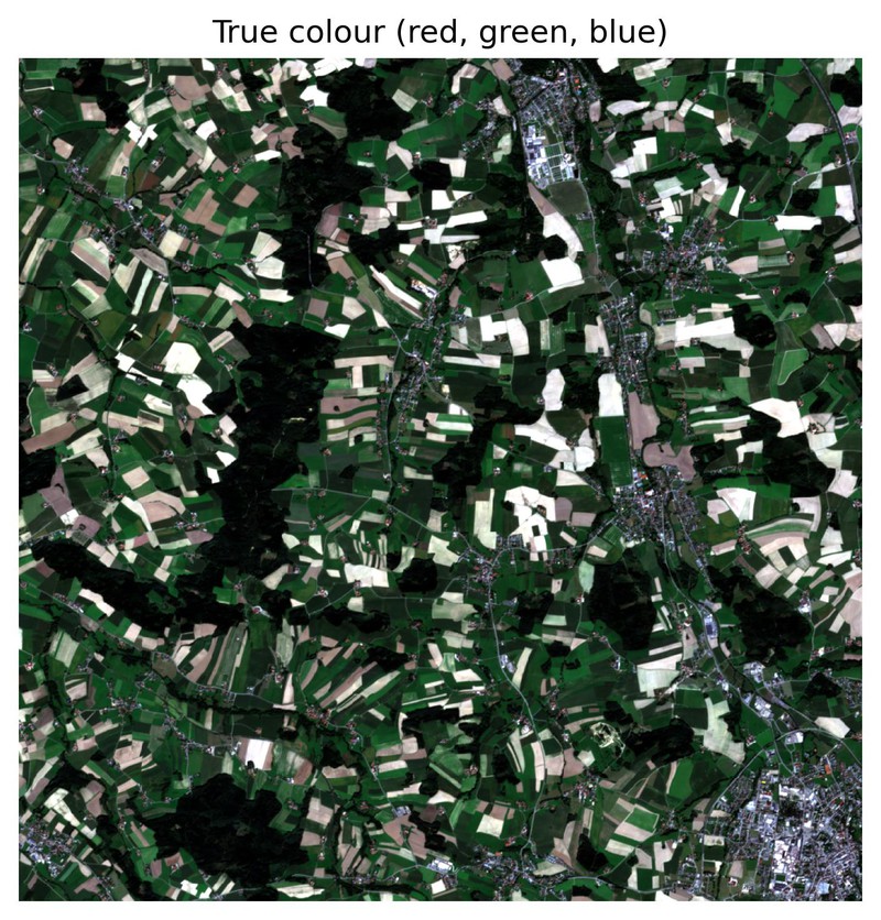
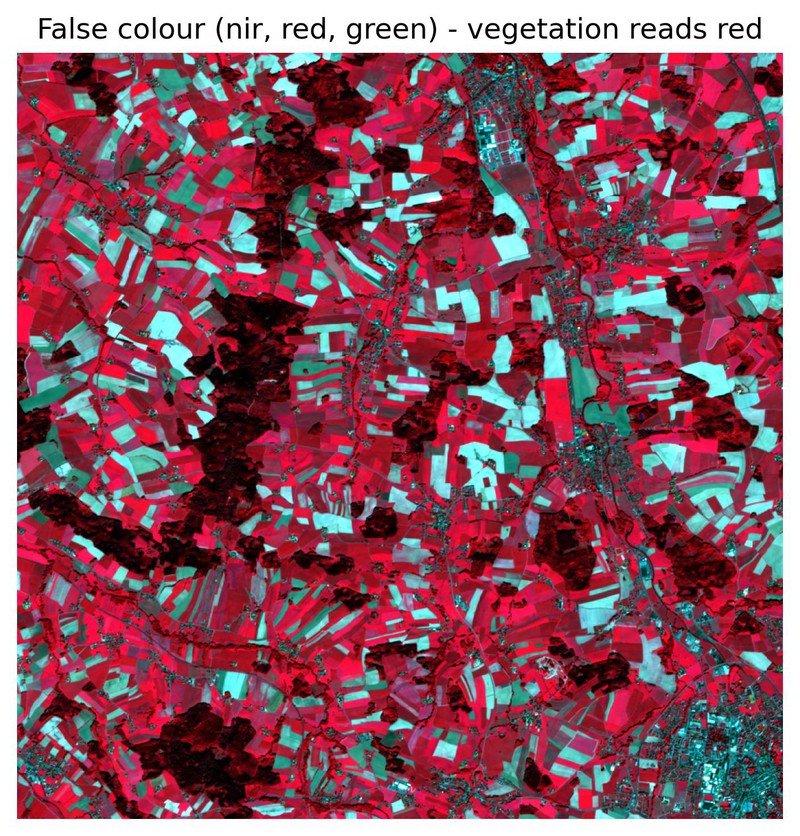
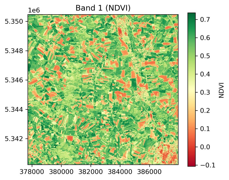
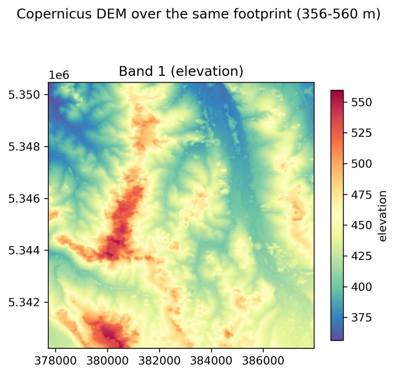
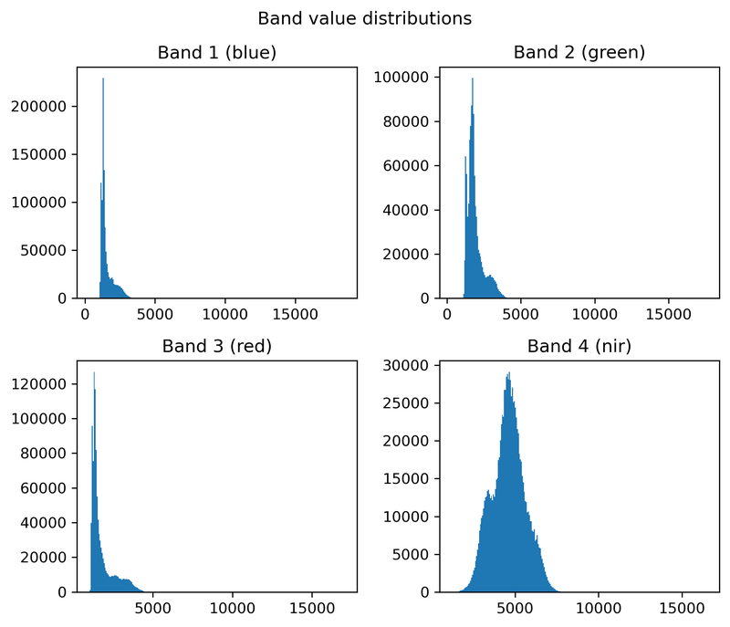
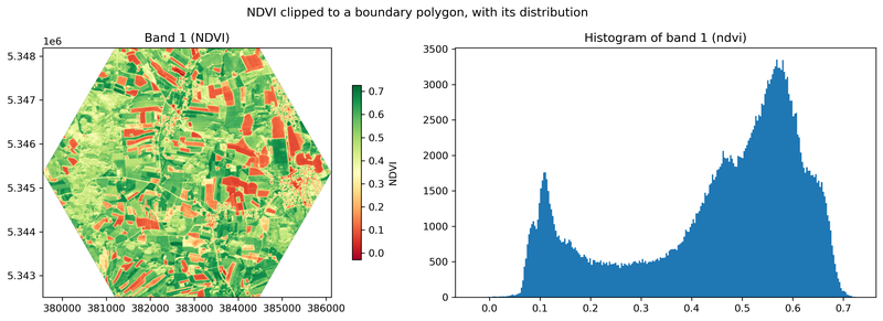
Every image below comes straight out of an Easy-EO plotting call on the sample
dataset, with the library's own defaults and no touch-ups. Regenerate them all
with python scripts/build_gallery.py.
 |
 |
scene.plot_composite(bands=["red", "green", "blue"]) |
scene.plot_composite(bands=["nir", "red", "green"]) |
 |
 |
scene.ndvi(red="red", nir="nir", name="NDVI").plot_raster(cmap="RdYlGn") |
dem.plot_raster(cmap="Spectral_r"), the same call on a DEM |
 |
 |
scene.plot_histogram(), every band at once |
clipped.plot_raster_with_histogram(cmap="RdYlGn") |
Bands are addressed by name throughout ("red", "nir") because the sample
carries band descriptions; a 1-based index works anywhere a name does.
Backends
One dataset type, with three backends underneath it:
| Backend | What it is for |
|---|---|
| Rasterio | Files and COGs GDAL can open, local or over HTTP, from load_raster() |
| NumPy | In-memory arrays with a CRS and transform attached, from load_array() and the product loaders |
| xarray + dask | Lazy, chunked reading of rasters larger than memory, from load_raster(path, chunks=...) (the lazy extra) |
Every operation, statistic and plot works on the Rasterio and lazy backends and
returns the same answer on both. On the NumPy backend, clipping, reprojecting,
mosaicking and stacking need a .to_rasterio() first, and the error says so.
See Backends for how they fit together.
Documentation
Full documentation, with user guides and the API reference: easy-eo.readthedocs.io
Citing Easy-EO
If Easy-EO contributes to published work, please cite it. The DOI
10.5281/zenodo.21967655 always
resolves to the latest release, and
CITATION.cff
drives GitHub's "Cite this repository" button. The
citation page has a
BibTeX entry, and a separate one for the sample dataset.
Project status
Active development. The API is stabilising but may change before v1.0, and every breaking change is listed under a Breaking heading in the changelog.
Contributing
Contributions are welcome: bug reports, feature requests and documentation
improvements as much as code. Please open an issue or pull request on GitHub,
and see CONTRIBUTING.md
for how to set up a development environment and run the checks. Report
security issues privately, as described in
SECURITY.md.
License
MIT License © 2025 Thomas Burns Botchwey
1 maintainer

Metadata
1 maintainer
Release files for easy-eo 0.6.0
For a detailed explanation of source distributions (sdists) and built distributions (wheels), please see the package formats documentation.
Source distribution (sdist)
| File | Size | Uploaded | |
|---|---|---|---|
| easy_eo-0.6.0.tar.gz | 198.1 kB | Details |
Built distribution (wheel)
| File | Interpreter | ABI | Platform | Reset |
|---|---|---|---|---|
| easy_eo-0.6.0-py3-none-any.whl | Python 3 | none | any | Details |
Total release size: 421.9 kB
Release files / easy_eo-0.6.0.tar.gz
| Download URL | easy_eo-0.6.0.tar.gz |
|---|---|
| Size | 198.1 kB |
| Tags | Source |
|
SHA-256 checksum How to use checksums |
b3da3ea55b6de23051d880dcc9bea56addb6089414e839b312548808870a67d7
|
|
BLAKE2b-256 checksum How to use checksums |
73fa5cb406cbb12ea70ea1cd23f06799510dce1ddb844c217341db56e4c71396
|
| Upload date | |
|
Uploaded using Trusted Publishing? What is trusted publishing? |
Yes |
| Uploaded via |
twine/7.0.0 CPython/3.13.14
|
Provenance
Provenance describes where a file came from. On PyPI, provenance is shared via attestations, which provide a verifiable record of the build or publishing details. View details, limitations and caveats.


PyPI Publish Attestation
PyPI verified that this artifact, at this checksum, originated from the publisher listed below.
Signed by GitHub Actions, verified by PyPI on Sep 28, 2026.
Transparency logRelease files / easy_eo-0.6.0-py3-none-any.whl
| Download URL | easy_eo-0.6.0-py3-none-any.whl |
|---|---|
| Size | 223.8 kB |
| Tags | Python 3 |
|
SHA-256 checksum How to use checksums |
c3cc20a50d86817e1cde733dc73b0b005ffb8fb68ad823b63e9ca6e711deb137
|
|
BLAKE2b-256 checksum How to use checksums |
365c6c8cf8242b4ef6f46ae0db060adb2827086dd510eb21d95ef5e085ac4ee0
|
| Upload date | |
|
Uploaded using Trusted Publishing? What is trusted publishing? |
Yes |
| Uploaded via |
twine/7.0.0 CPython/3.13.14
|
Provenance
Provenance describes where a file came from. On PyPI, provenance is shared via attestations, which provide a verifiable record of the build or publishing details. View details, limitations and caveats.
PyPI Publish Attestation
PyPI verified that this artifact, at this checksum, originated from the publisher listed below.
Signed by GitHub Actions, verified by PyPI on Sep 28, 2026.
Transparency log













