A Python toolkit for producing publication-quality microeconomics diagrams.

Project description
econ-viz


A Python toolkit for producing publication-quality microeconomics diagrams. Define utility functions declaratively, solve for consumer equilibria, and export figures as raster images or LaTeX/TikZ source — all in a few lines of code.
Installation
pip install econ-viz
Requires Python 3.12 or later.
Quick Start
import numpy as np
from econ_viz import Canvas, levels, solve
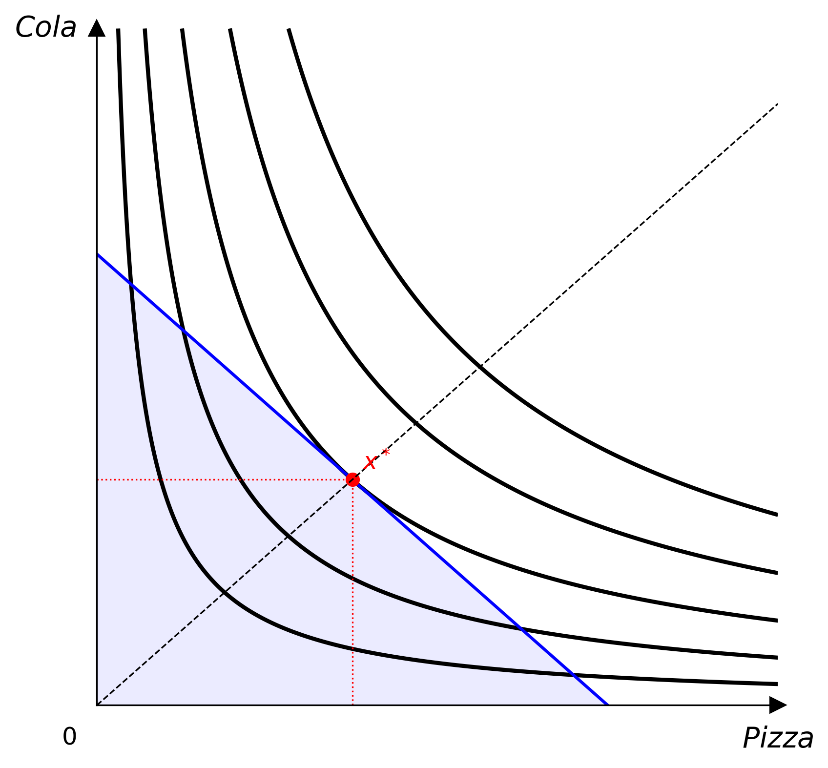
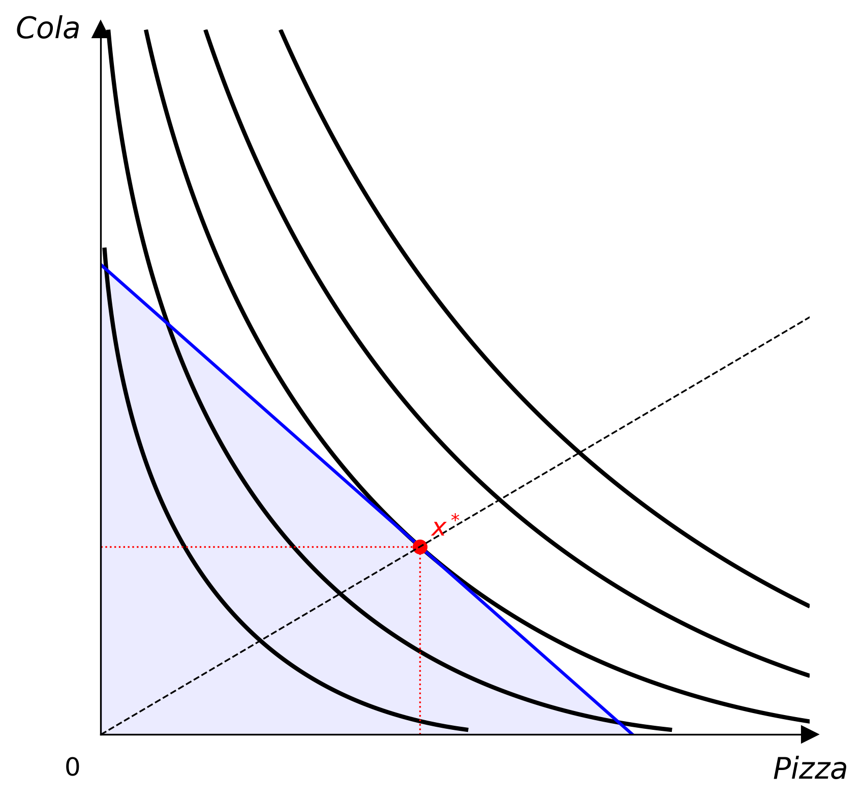
from econ_viz.models import CobbDouglas
model = CobbDouglas(alpha=0.5, beta=0.5)
eq = solve(model, px=2.0, py=3.0, income=30.0)
lvls = levels.around(eq.utility, n=5)
cvs = Canvas(x_max=20, y_max=15, x_label="x", y_label="y",
title="Cobb-Douglas $x^{0.5} y^{0.5}$")
cvs.add_utility(model, levels=lvls)
cvs.add_budget(2.0, 3.0, 30.0, fill=True)
cvs.add_equilibrium(eq, show_ray=True)
cvs.save("cobb_douglas.png")
Utility Models
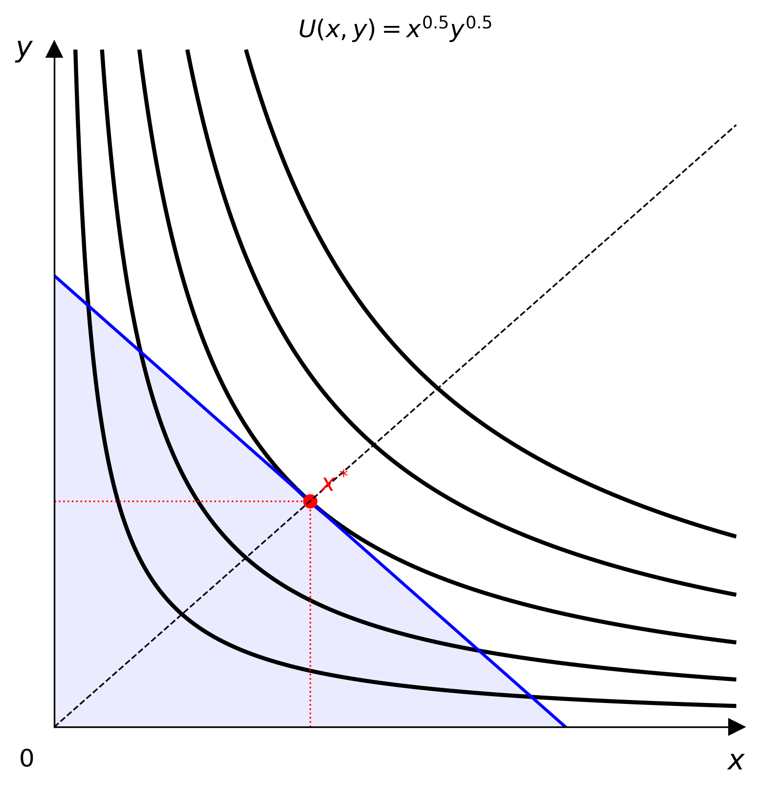
Cobb-Douglas
from econ_viz.models import CobbDouglas

model = CobbDouglas(alpha=0.3, beta=0.7)
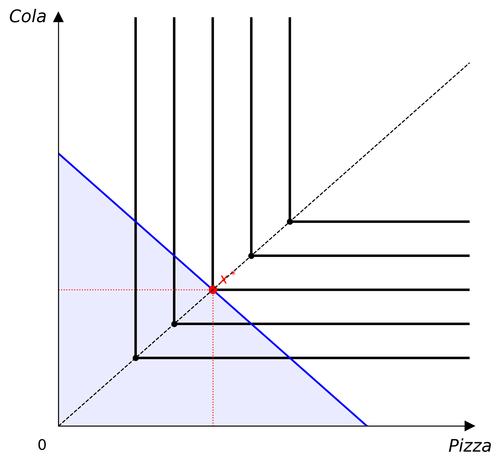
Leontief (Perfect Complements)
from econ_viz.models import Leontief

model = Leontief(a=1.0, b=1.0)   # U = min(ax, by)
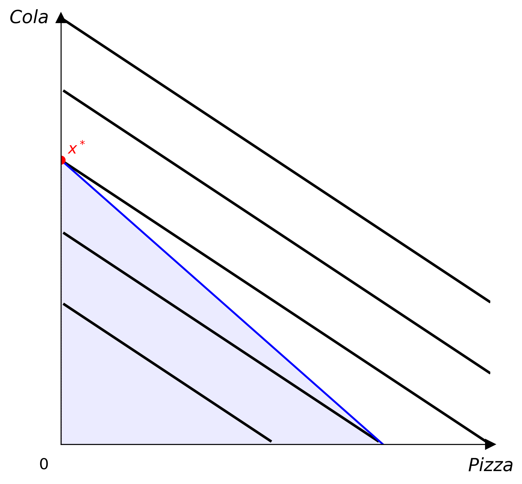
Perfect Substitutes
from econ_viz.models import PerfectSubstitutes

model = PerfectSubstitutes(a=1.0, b=2.0)   # U = ax + by
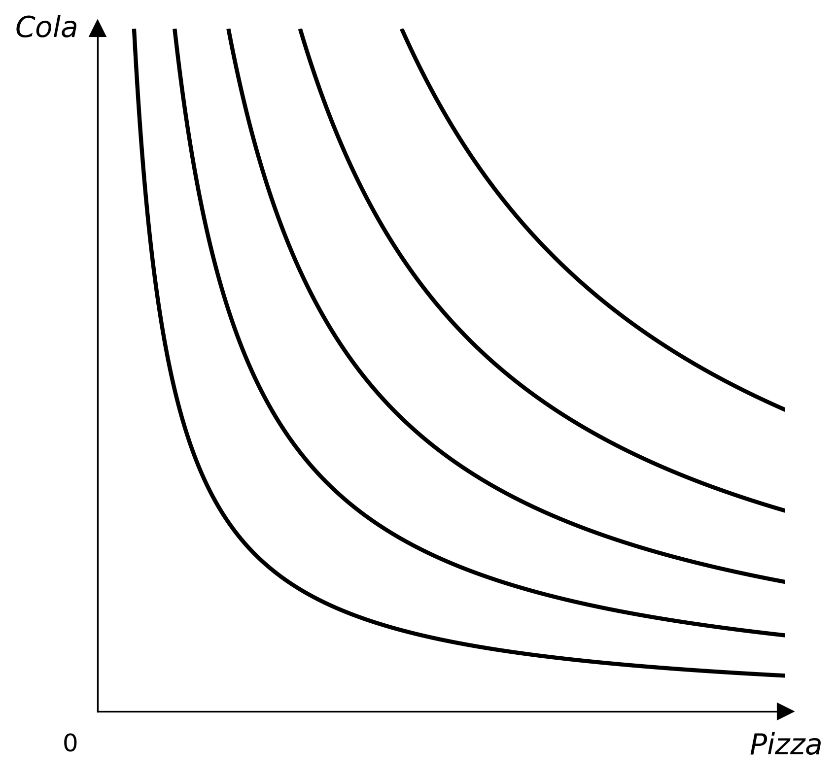
CES
from econ_viz.models import CES

model = CES(rho=-0.5, alpha=0.5)   # elasticity of substitution = 1/(1+rho)
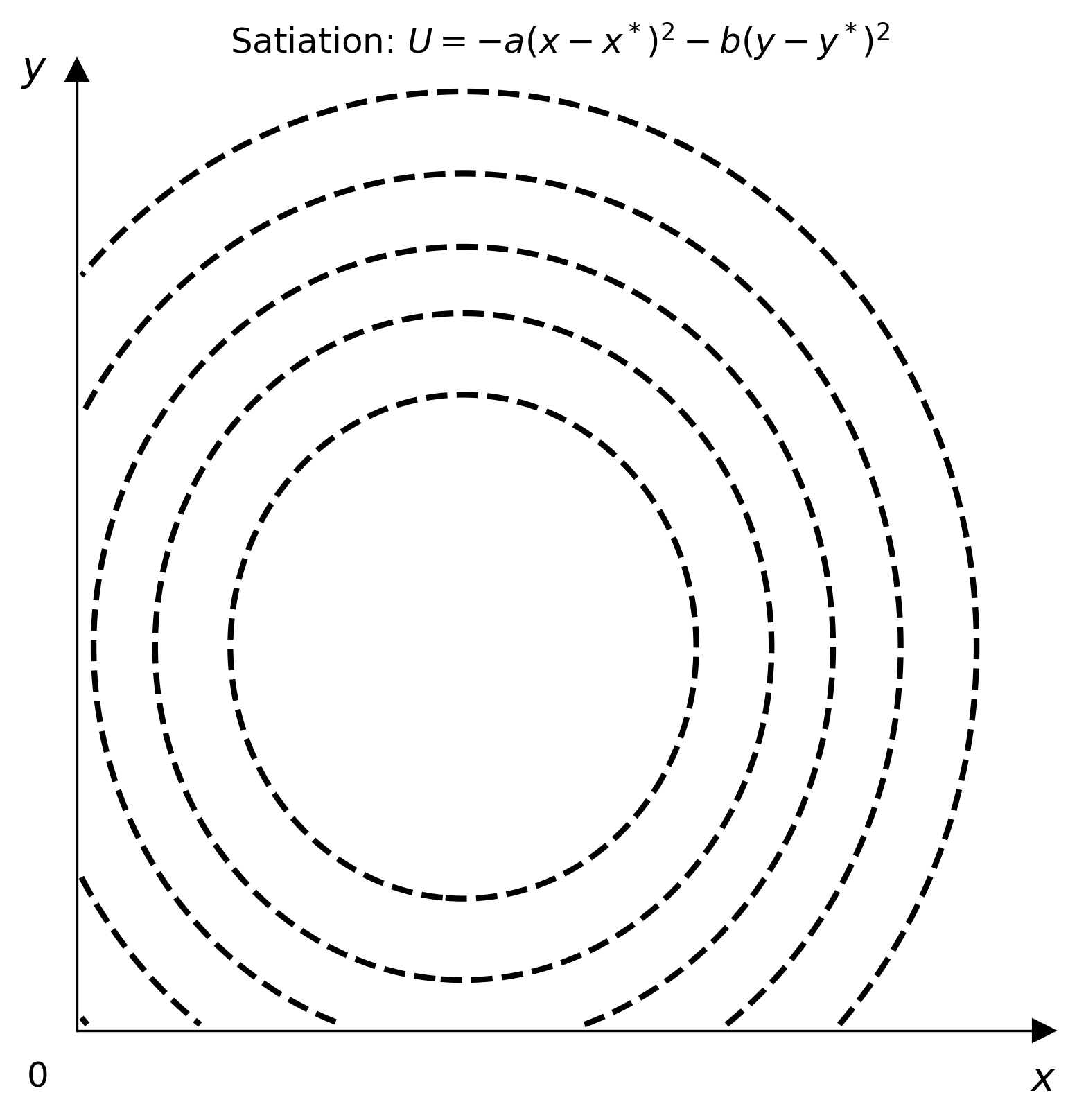
Satiation (Bliss Point)
from econ_viz.models import Satiation

model = Satiation(bliss_x=6.0, bliss_y=4.0, a=1.0, b=1.0)
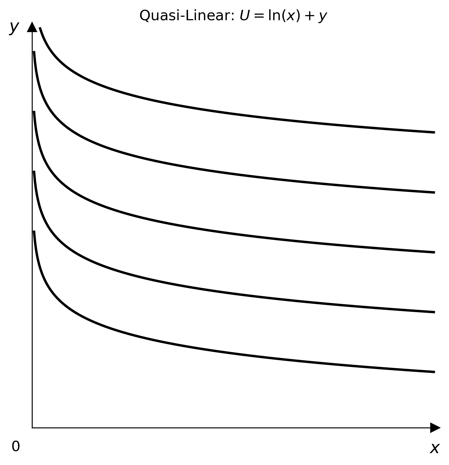
Quasi-Linear
import numpy as np
from econ_viz.models import QuasiLinear

model = QuasiLinear(v_func=np.log, linear_in="y")   # U = log(x) + y
LaTeX Input
Parse standard LaTeX math expressions directly into model instances:
from econ_viz import parse_latex

cd  = parse_latex(r"x^{0.4} y^{0.6}")
leo = parse_latex(r"\min(2x, 3y)")
ps  = parse_latex(r"2x + 3y")
The parser accepts common preambles such as U(x,y) =, U =, and bare expressions. Unrecognised patterns raise ParseError.
Advanced Models
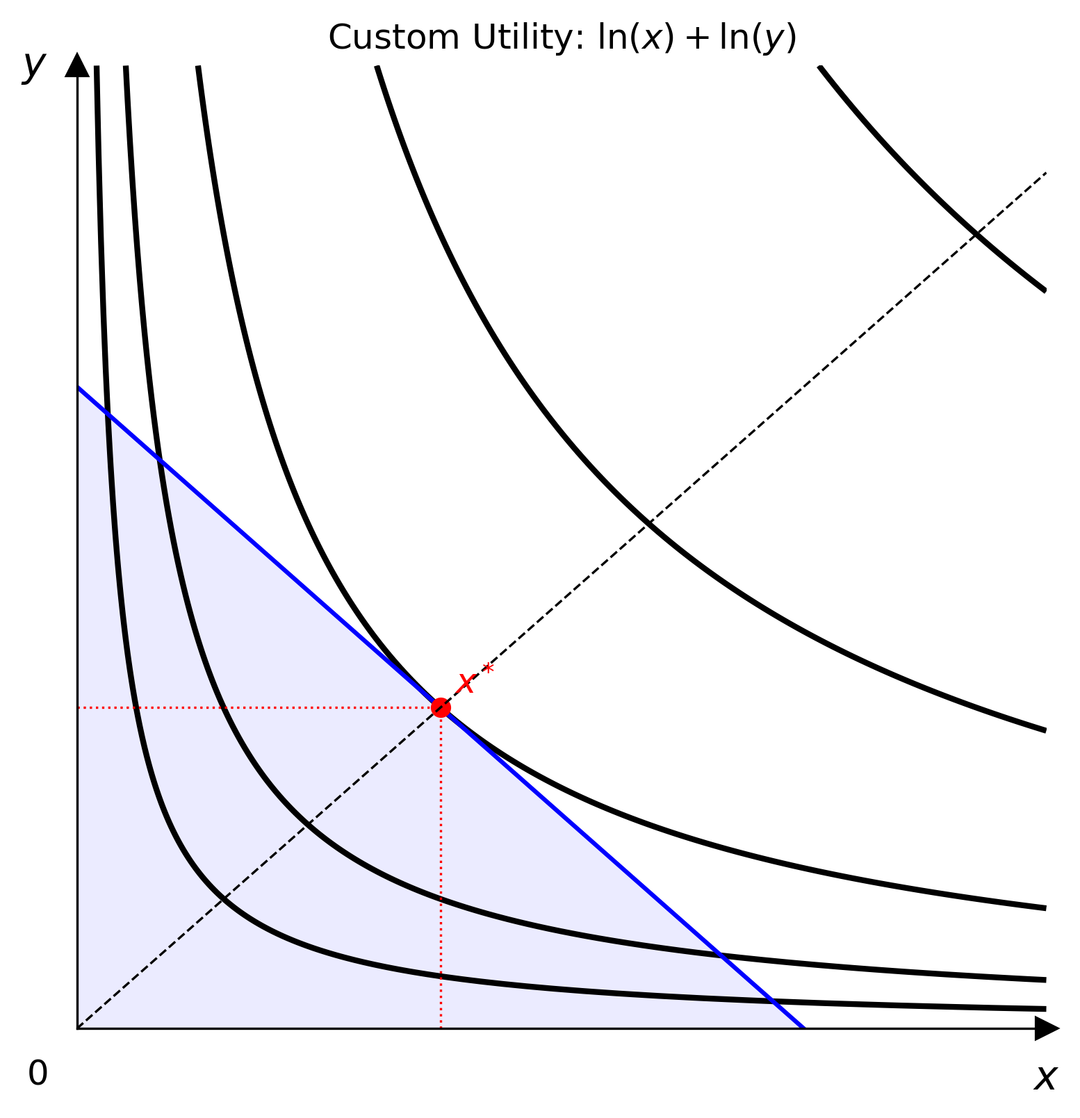
Custom Utility
Wrap any vectorised Python callable as a first-class model. The callable is validated at construction time against a random NumPy mesh-grid.
import numpy as np
from econ_viz.models import CustomUtility

model = CustomUtility(func=lambda x, y: np.log(x) + np.log(y), name="log+log")
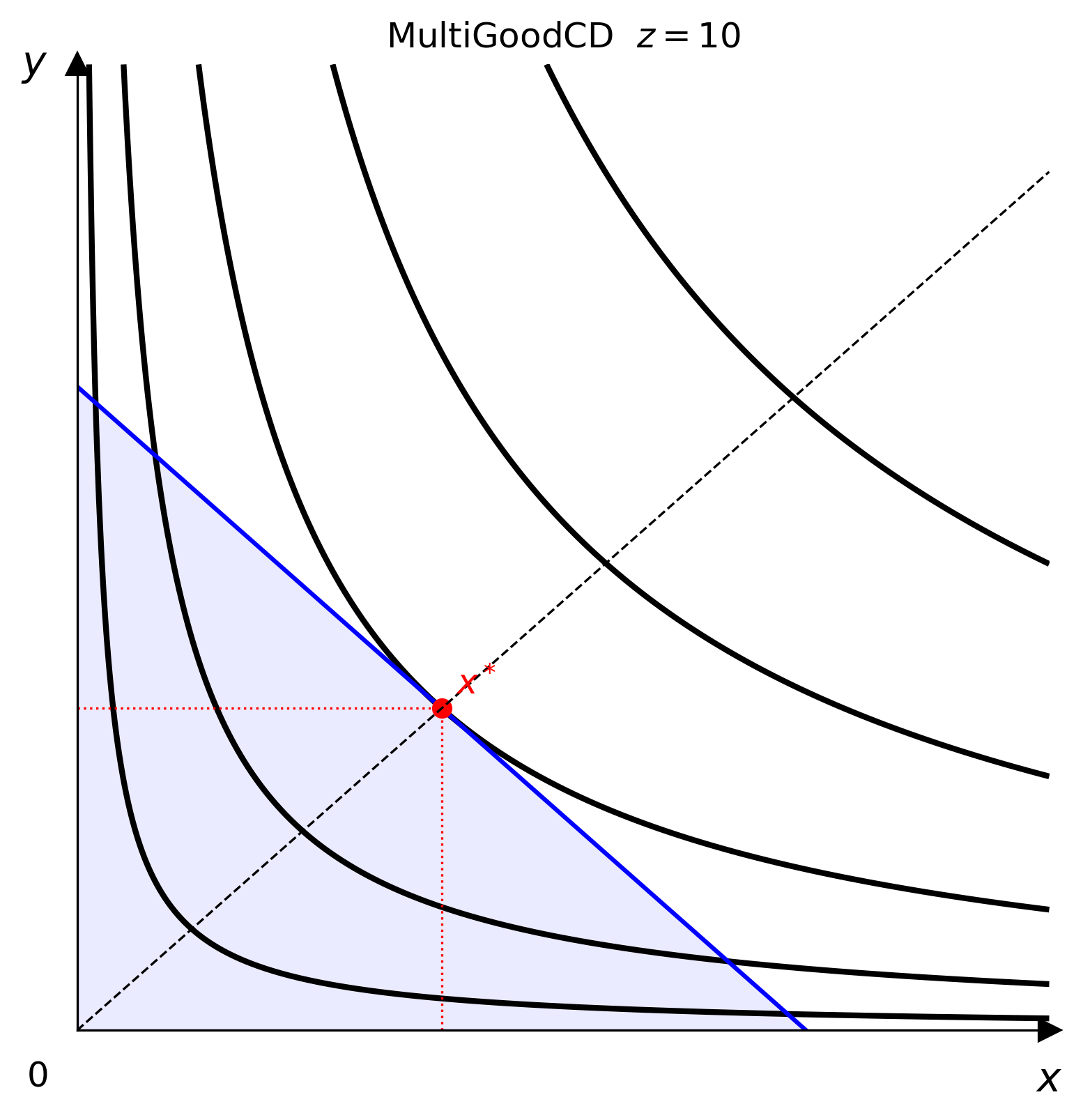
Multi-Good Cobb-Douglas
Model preferences over N goods and project to a 2-D canvas via freeze():
from econ_viz.models import MultiGoodCD

m3   = MultiGoodCD({'x': 0.3, 'y': 0.3, 'z': 0.4})
flat = m3.freeze(z=10.0)   # returns a CustomUtility ready for Canvas
from econ_viz import Canvas, levels, solve

eq   = solve(flat, px=2.0, py=3.0, income=30.0)
lvls = levels.around(eq.utility, n=5)

cvs = Canvas(x_max=20, y_max=15, title=r"MultiGoodCD  $z=10$")
cvs.add_utility(flat, levels=lvls)
cvs.add_budget(2.0, 3.0, 30.0, fill=True)
cvs.add_equilibrium(eq)
cvs.save("multigood.png")
Solving for Equilibrium
solve() returns an Equilibrium named tuple with fields x, y, and utility:
from econ_viz import solve
from econ_viz.models import CobbDouglas

eq = solve(CobbDouglas(), px=2.0, py=3.0, income=30.0)
print(eq.x, eq.y, eq.utility)
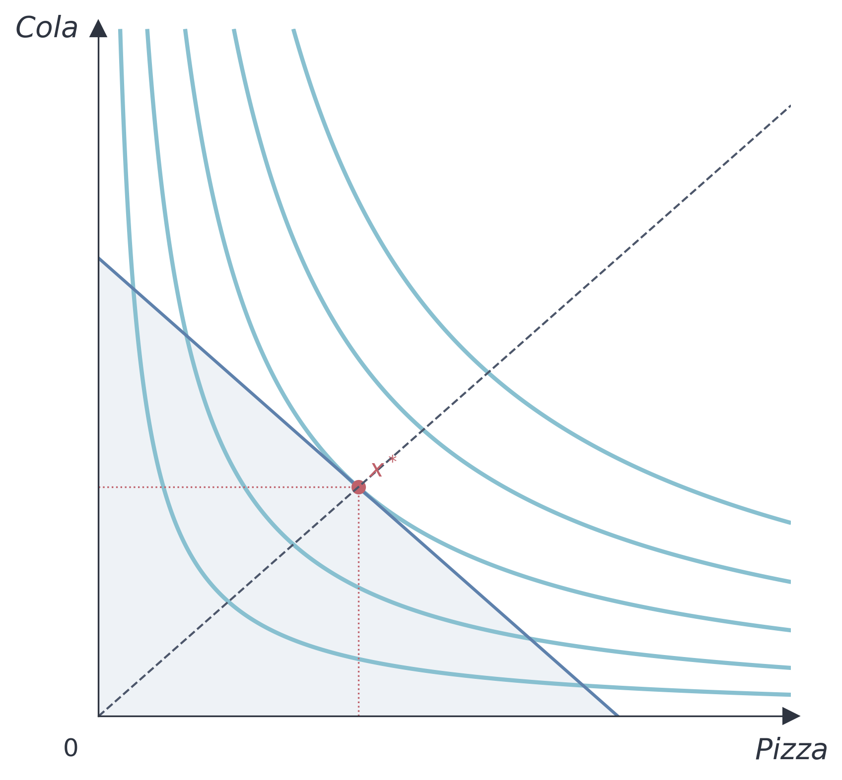
Themes
from econ_viz import Canvas, themes

cvs = Canvas(x_max=20, y_max=15)                    # default theme
cvs = Canvas(x_max=20, y_max=15, theme=themes.nord) # nord theme
| Default | Nord |
|---|---|
 |
 |
Export
cvs.save("figure.png")    # raster (DPI controlled by Canvas(dpi=300))
cvs.save("figure.tikz")   # TikZ/PGFPlots source for LaTeX
License
MIT © Anthony Sung
Release history Release notifications | RSS feed


Download files
Download the file for your platform. If you're not sure which to choose, learn more about installing packages.
Source Distribution
Built Distribution
Filter files by name, interpreter, ABI, and platform.
If you're not sure about the file name format, learn more about wheel file names.
Copy a direct link to the current filters
File details
Details for the file econ_viz-0.1.2.tar.gz.
File metadata
- Download URL: econ_viz-0.1.2.tar.gz
- Upload date:
- Size: 22.9 kB
- Tags: Source
- Uploaded using Trusted Publishing? No
- Uploaded via: poetry/2.3.2 CPython/3.13.12 Linux/6.17.0-19-generic
File hashes
| Algorithm | Hash digest | |
|---|---|---|
| SHA256 |
300f6546f25cfe985d33caa24435d728aa69b7d4982aeee04635528fcb74fa15
|
|
| MD5 |
dc4de96afba2e634cdb449bf8afeaa3b
|
|
| BLAKE2b-256 |
412fd133b6ee9a7fd76d7c40df0de5a33d80e67d5a6495d5b1d13a95ef54f5c1
|
File details
Details for the file econ_viz-0.1.2-py3-none-any.whl.
File metadata
- Download URL: econ_viz-0.1.2-py3-none-any.whl
- Upload date:
- Size: 30.7 kB
- Tags: Python 3
- Uploaded using Trusted Publishing? No
- Uploaded via: poetry/2.3.2 CPython/3.13.12 Linux/6.17.0-19-generic
File hashes
| Algorithm | Hash digest | |
|---|---|---|
| SHA256 |
605e91ef895a561df654ff2b0151254ec5761fbe15f20be4f7fdae9db38a2ae9
|
|
| MD5 |
a4edce064a2af3a07113c48cb3fe2721
|
|
| BLAKE2b-256 |
e4b1e0493b333a0d18b217d5b3c1c42db9c113f725681bd9869682c2633d4ee6
|


