

ENFORCE - Nonlinear Constrained Learning with Adaptive-depth Neural Projection
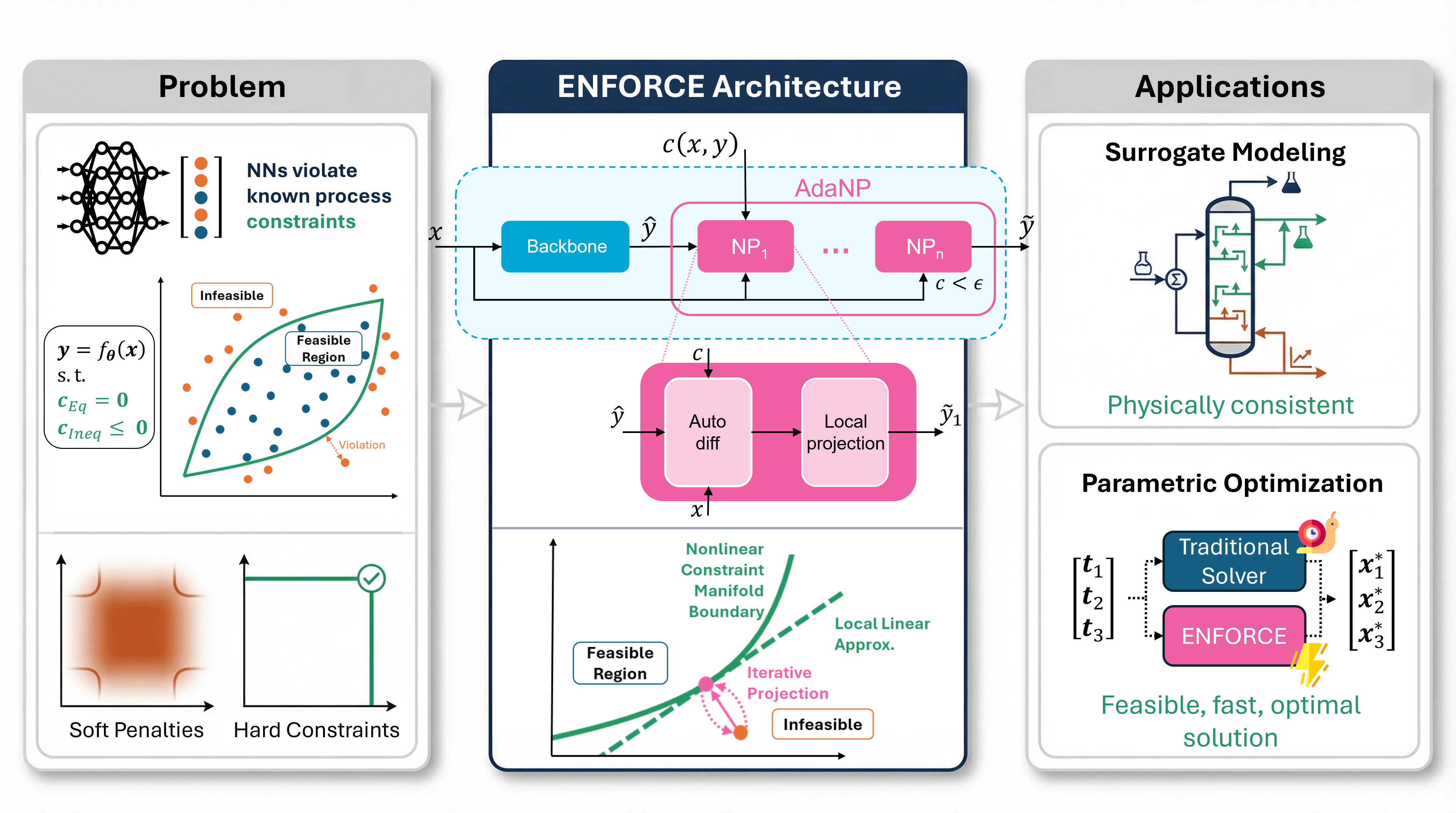


Nonlinear Constrained Learning with Adaptive-depth Neural Projection.
ENFORCE combines a neural network backbone with an AdaNP (Adaptive-depth Neural Projection) module to drive predictions toward feasibility with respect to nonlinear equality and inequality constraints. At each forward pass, AdaNP iteratively applies a linearize-and-project correction - an SQP-inspired Gauss-Newton step - until the constraint residual falls below a prescribed tolerance ε.
For equality constraints that are affine in the output y, a single NP step achieves exact feasibility. For general nonlinear constraints, ε-feasibility is obtained locally: under standard regularity conditions (LICQ, C² smoothness) and when the backbone prediction is sufficiently close to the constraint manifold, AdaNP reduces the residual ‖c(x,ỹ)‖ below ε with a linear convergence rate. The model is trained with standard unconstrained optimization (Adam), not constrained solvers.
Inequality constraints g(x,y) ≤ 0 are handled via a Fischer-Burmeister (FB) reformulation that converts them into equalities in an extended output space [y, λ], so the same AdaNP projection applies without modification.
Reference
If you use ENFORCE in your work, please cite the paper:
@Article{Lastrucci2025_ENFORCENonlinearConstrained,
  author    = {Lastrucci, Giacomo and Schweidtmann, Artur M.},
  journal   = {arXiv preprint arXiv:2502.06774},
  title     = {ENFORCE: Nonlinear Constrained Learning with Adaptive-depth Neural Projection},
  year      = {2025},
  copyright = {arXiv.org perpetual, non-exclusive license},
  doi       = {10.48550/arXiv.2502.06774},
  keywords  = {Machine Learning (cs.LG), FOS: Computer and information sciences},
  publisher = {arXiv},
}
To refer to a specific version of the software, cite the repository: the "Cite this repository" button on GitHub gives the metadata from CITATION.cff, including the version.
Installation
Requires Python ≥ 3.10 and PyTorch ≥ 2.0.
pip
PyTorch is a dependency of ENFORCE. Install the PyTorch build for your hardware first, following the PyTorch installation guide; pip then keeps it. Otherwise pip installs PyTorch from PyPI (the CUDA build on Linux, the CPU build on Windows and macOS).
# 1. PyTorch for your hardware, e.g.
pip install torch --index-url https://download.pytorch.org/whl/cpu      # CPU
pip install torch --index-url https://download.pytorch.org/whl/cu126    # CUDA 12.6

# 2. ENFORCE
pip install enforce-nn
The tutorial notebooks and benchmark scripts also need matplotlib and pandas, included in the examples extra:
pip install "enforce-nn[examples]"
uv
uv add enforce-nn
In your own project, uv resolves PyTorch from PyPI like pip. To use a specific PyTorch build, set the PyTorch index in your project's pyproject.toml (see uv's PyTorch guide), e.g. for CPU:
[tool.uv.sources]
torch = [{ index = "pytorch-cpu" }]

[[tool.uv.index]]
name = "pytorch-cpu"
url = "https://download.pytorch.org/whl/cpu"
explicit = true
From source (development)
git clone https://github.com/process-intelligence-research/ENFORCE
cd ENFORCE
uv sync    # package, examples and dev tools
In this repository, uv sync takes PyTorch from the CPU index set in its pyproject.toml; for CUDA, change that index URL (e.g. to https://download.pytorch.org/whl/cu126). This setting applies only when working in the repository, not to the published package. With pip instead: install PyTorch as above, then pip install -e ".[examples]".
Quick start
Supervised - nonlinear equality constraint
Fit x → (y₁, y₂) subject to the nonlinear constraint (0.5 y₁)² + x² + y₂ = 0:
import numpy as np
import torch
from enforce import Scaler, Constraints, ENFORCE, ENFORCEConfig, ENFORCELoss, ENFORCELossConfig
from enforce.models import MLPConfig, ENFORCEConstrainedMLP
from enforce.engines import Trainer, TrainingConfig, Evaluator, EvaluationConfig
from enforce.data import scale_data

np.random.seed(0)  # data; initial weights: MLPConfig.random_seed, shuffling: TrainingConfig.random_seed

# 1. Data
def make_data(n):
    x = np.random.uniform(-1.0, 1.0, (n, 1))
    return x, np.column_stack([2 * np.sin(5 * x[:, 0]), -(np.sin(5 * x[:, 0]) ** 2 + x[:, 0] ** 2)])

x_train, y_train = make_data(500)
x_test,  y_test  = make_data(200)
x_tr_s, y_tr_s, x_te_s, y_te_s, sp = scale_data(x_train, y_train, x_test, y_test)
x_tr_t, y_tr_t, x_te_t, y_te_t = (torch.tensor(a, dtype=torch.float32) for a in (x_tr_s, y_tr_s, x_te_s, y_te_s))
scaler = Scaler((sp["input_mean"], sp["input_std"]), (sp["output_mean"], sp["output_std"]))

# 2. Constraint c(x, y) = 0  (operates on unscaled x and y, returns [BS])
def my_constraint(x, y):
    return (0.5 * y[:, 0]) ** 2 + x[:, 0] ** 2 + y[:, 1]

constraints = Constraints(c=[my_constraint])

# 3. Build: loss, ENFORCE layer, backbone
loss  = ENFORCELoss(scaler, constraints, ENFORCELossConfig(weight_loss_displacement=0.5))
layer = ENFORCE(scaler, constraints, loss, ENFORCEConfig(training_tolerance=1e-4, inference_tolerance=1e-6, max_it=100))
model = ENFORCEConstrainedMLP(MLPConfig(input_neurons=1, hidden_neurons=64, output_neurons=2, hidden_layers=1), layer)

# 4. Train / evaluate
model  = Trainer(model, loss, scaler, constraints, TrainingConfig(epochs=2000)).fit(x_tr_t, y_tr_t)
result = Evaluator(model, loss, scaler, constraints, EvaluationConfig()).evaluate(x_te_t, y_te_t)

preds = result.predictions  # shape [N, 2], already unscaled
print(f"max |c(x, y)|: {result.metrics['residual_max']:.1e}")  # below inference_tolerance = 1e-6
Each item in c (equalities) or g (inequalities) is either a plain callable returning one constraint [BS], or a Constraint block of several constraints evaluated together. Equations with the same structure are fastest as one vectorised block, optionally with an analytical Jacobian jac(x, y) -> [BS, size, NO]:
from enforce import Constraint, Constraints
import torch

A = torch.tensor([[1.0, 2.0], [0.0, 1.0]])  # equations A y = x, [size, NO]
constraints = Constraints(c=[Constraint(lambda x, y: y @ A.T - x, size=A.shape[0], jac=lambda x, y: A.expand(len(y), -1, -1))])
Self-supervised - parametric optimization with inequality
For each x ∈ [2, 4], minimize ‖y‖² subject to y₁² + y₂ = x (equality) and y₁ ≥ 0 (inequality via FB):
import numpy as np
import torch
from enforce import Scaler, Constraints, ENFORCE, ENFORCEConfig, ENFORCELossConfig
from enforce.losses import ENFORCESSLLoss
from enforce.models import MLPConfig, ENFORCEConstrainedMLP
from enforce.engines import Trainer, TrainingConfig, Evaluator, EvaluationConfig
from enforce.data import scale_data

np.random.seed(0)  # data; initial weights: MLPConfig.random_seed, shuffling: TrainingConfig.random_seed

# 1. Constraints: equality c(x, y) = 0 and inequality g(x, y) <= 0
def parabola(x, y):  return y[:, 0] ** 2 + y[:, 1] - x[:, 0]
def g_nonneg(x, y):  return -y[:, 0]   # y1 >= 0  =>  g = -y1 <= 0

constraints = Constraints(c=[parabola], g=[g_nonneg])

# 2. SSL objective - minimize ||y||² (yhat = [y, λ]: drop the FB multiplier column)
class MinNorm(ENFORCESSLLoss):
    def ssl_loss(self, x, yhat):
        return torch.mean(torch.sum(yhat[:, :2] ** 2, dim=1))

# 3. Dummy labels (no targets needed in self-supervised mode), extended with one zero λ column per inequality
N = 2000
x_train = np.random.uniform(2.0, 4.0, (N, 1)).astype(np.float32)
y_dummy = constraints.extend_outputs(np.zeros((N, 2), dtype=np.float32))
x_tr_s, y_tr_s, _, _, sp = scale_data(x_train, y_dummy, x_train, y_dummy)
x_tr_t, y_tr_t = torch.tensor(x_tr_s), torch.tensor(y_tr_s)
scaler = Scaler((sp["input_mean"], sp["input_std"]), (sp["output_mean"], sp["output_std"]))

# 4. Build - the backbone predicts y only (scaler.no - constraints.ng = 2); λ is appended by ENFORCE
loss  = MinNorm(scaler, constraints, ENFORCELossConfig(weight_loss_displacement=0.5))
layer = ENFORCE(scaler, constraints, loss, ENFORCEConfig(training_tolerance=1e-4, inference_tolerance=1e-6, max_it=100))
mlp_cfg = MLPConfig(input_neurons=1, hidden_neurons=64, output_neurons=scaler.no - constraints.ng, hidden_layers=2)
model = ENFORCEConstrainedMLP(mlp_cfg, layer)

# 5. Train / evaluate
model  = Trainer(model, loss, scaler, constraints, TrainingConfig(epochs=2000)).fit(x_tr_t, y_tr_t)
result = Evaluator(model, loss, scaler, constraints, EvaluationConfig()).evaluate(x_tr_t, y_tr_t)
preds  = result.predictions  # [N, 2] - y1, y2 only (multipliers removed)
print(f"max |c(x, y)|: {result.metrics['residual_max']:.1e}, "  # below inference_tolerance = 1e-6
      f"max g(x, y) violation: {result.metrics['ineq_g1_max_violation']:.1e}")  # 0 if feasible
Tutorials
Step-by-step notebooks in the notebooks/tutorials/ folder:
| Notebook | Topic |
|---|---|
01_equality_constraints.ipynb |
Supervised fitting with a nonlinear equality constraint (unit circle) |
02_inequality_constraints.ipynb |
Supervised fitting with inequality bounds via Fischer-Burmeister |
03_parametric_optimization.ipynb |
Self-supervised parametric optimization - mixed equality + inequality, MLP comparison |
How it works
ENFORCE appends an AdaNP module to any backbone network. Each NP layer solves a linearized QP: given the backbone output ŷ and the constraint Jacobian B = ∂c/∂y|_{x,ŷ}, the closed-form correction step is
ỹ = (I − Bᵀ(BBᵀ)⁻¹B) ŷ + Bᵀ(BBᵀ)⁻¹v, with v = Bŷ − c(x, ŷ)
This is the solution to the locally linearized projection problem and corresponds to a Gauss-Newton SQP step (without Hessian of constraints). AdaNP stacks NP layers adaptively until ‖c(x, ỹ)‖ < ε or max_it is reached, relinearizing at each iterate. The Jacobian B is computed via automatic differentiation through the constraint function c only (not the backbone), or taken from an analytical Jacobian given with the constraint, so the per-step cost is O(N_C³).
Scope of the ε-feasibility claim. For equality constraints affine in y, a single NP step achieves exact feasibility. Inequalities are reformulated with the Fischer-Burmeister function, which is nonlinear even for affine g, so they may need more steps. For nonlinear constraints, convergence is local: it requires the backbone prediction to lie in a neighborhood of the constraint manifold where LICQ holds and the linearization is accurate. If the backbone is far from feasibility or the Jacobian is ill-conditioned, residuals may remain above ε within the depth cap.
Inequality constraints g(x,y) ≤ 0 are reformulated using the Fischer-Burmeister function
φ_FB(λᵢ, −gᵢ) = √(λᵢ² + gᵢ² + ε_FB) − λᵢ + gᵢ = 0
which encodes the KKT complementarity conditions as an equality. AdaNP then operates in the extended space [y, λ] without any modification to the core algorithm.
Training. ENFORCE is trained with standard Adam on a loss ℓ = ℓ_task + λ_D ‖ŷ − ỹ‖² + λ_C ‖c(x,ỹ)‖, where the displacement penalty λ_D ‖ŷ − ỹ‖² encourages the backbone to produce predictions already close to the constraints manifold, reducing the depth needed at inference. An adaptive activation heuristic (inspired by trust-region methods) enables AdaNP only when the projection improves a task-specific loss measure, providing an automatic warm-up phase before constrained learning begins.
Reproducing paper results
The original benchmark datasets can be downloaded from here and placed in data/raw. The original benchmark training results can be downloaded from here (7.6 GB).
All benchmarks are run through scripts/run_benchmark.py. Select the problem by setting PROBLEM in benchmark_problems/config_benchmarking.py, then run from the repo root:
python scripts/run_benchmark.py
Function fitting (equality constraint)
# benchmark_problems/config_benchmarking.py
PROBLEM = "function_fitting"
MODEL   = "BOTH"   # trains ENFORCE and MLP baseline
To reproduce the hyperparameter study (sweep over λ_D and ε_T):
bash scripts/run_hyperparameter_study.sh
Function fitting with inequality constraints
PROBLEM = "sin_ineq"
MODEL   = "BOTH"
Engineering case studies
PROBLEM = "extraction_column"   # extractive distillation surrogate
# or
PROBLEM = "pooling"             # pooling problem (equality + inequality)
MODEL   = "BOTH"
Both require the datasets from Iftakher et al.. Download it from here. Place the CSV files under data/raw/<problem>/ as expected by the data paths in config_benchmarking.py.
Parametric optimization benchmarks
PROBLEM = "nonconvex_linear"     # nonconvex objective, linear equality constraints
# or
PROBLEM = "nonconvex_nonlinear"  # nonconvex objective, nonlinear equality constraints
MODEL   = "ENFORCE"
These problems require pre-generated data files. Download them and place them under data/raw/<problem>/ following the filenames in config_benchmarking.py. Data can be generated from the DC3 repository.
General settings
Key flags in benchmark_problems/config_benchmarking.py:
| Flag | Default | Effect |
|---|---|---|
MODEL |
"BOTH" |
"ENFORCE", "MLP", or "BOTH" |
N |
5 |
number of independent runs |
PLOT |
True |
save result figures |
SAVE |
True |
save model weights and metrics |
FIX_SEED |
False |
fix random seed across runs |
Contributing and support
Questions, bug reports and feature requests go to GitHub issues. To contribute code, see CONTRIBUTING.md for the development setup, the checks to run and how to open a pull request.
Contributors
 |
Giacomo Lastrucci |   |
 |
Daniel Schicksnus | |
 |
Artur M. Schweidtmann | |
Acknowledgements
This research is supported by Shell Global Solutions International B.V., for which we express sincere gratitude.
License
This work is licensed under a MIT license - see LICENSE.
Technische Universiteit Delft hereby disclaims all copyright interest in the program “ENFORCE” written by Artur M. Schweidtmann. Paulien Herder, Dean of Applied Science
Copyright (C) 2025 Artur Schweidtmann, TU Delft
👨💼 Contact & Support
Dr. Artur Schweidtmann
Process Intelligence Research
TU Delft
Connect with us:


Built with ❤️ by the Process Intelligence Research team at TU Delft
2 maintainers


Metadata
2 maintainers
Release files for enforce-nn 2.0.0
For a detailed explanation of source distributions (sdists) and built distributions (wheels), please see the package formats documentation.
Source distribution (sdist)
| File | Size | Uploaded | Provenance | Actions |
|---|---|---|---|---|
| enforce_nn-2.0.0.tar.gz | 8.9 MB | Without provenance | Details for enforce_nn-2.0.0.tar.gz |
Built distribution (wheel)
| File | Interpreter | ABI | Platform | Actions Reset |
|---|---|---|---|---|
| enforce_nn-2.0.0-py3-none-any.whl | Python 3 | none | any | Details for enforce_nn-2.0.0-py3-none-any.whl |
Total release size: 9.0 MB
Release files / enforce_nn-2.0.0.tar.gz
| Download URL | enforce_nn-2.0.0.tar.gz |
|---|---|
| Size | 8.9 MB |
| Tags | Source |
|
SHA-256 checksum How to use checksums |
fc91dc7b38b8d362b222e2f7540078b32b8896a1df4bb5d9b62c24b8995f36b6
|
|
BLAKE2b-256 checksum How to use checksums |
fcd2624598374fe4018ea9103b0fe527286f6939e5f93ef58bdaee83362cf027
|
| Upload date | |
|
Uploaded using Trusted Publishing? What is trusted publishing? |
No |
| Uploaded via |
twine/7.0.0 CPython/3.12.11
|
Release files / enforce_nn-2.0.0-py3-none-any.whl
| Download URL | enforce_nn-2.0.0-py3-none-any.whl |
|---|---|
| Size | 40.4 kB |
| Tags | Python 3 |
|
SHA-256 checksum How to use checksums |
c812fbc3675a2085f8643329e07fc2350b758ee978ea32e4e2f8c723ff460580
|
|
BLAKE2b-256 checksum How to use checksums |
ee965bac04cd9073c3f78c6e3be4088c4355ac0e8055f952861a9ecbc488ebc5
|
| Upload date | |
|
Uploaded using Trusted Publishing? What is trusted publishing? |
No |
| Uploaded via |
twine/7.0.0 CPython/3.12.11
|
Security for enforce-nn 2.0.0
Provenance
Provenance describes where a file came from. On PyPI, provenance is shared via attestations, which provide a verifiable record of the build or publishing details. View details, limitations and caveats.
No provenance found
None of the files in this release were uploaded with provenance metadata.
A note on package security
PyPI is a repository for distributing packages, not a service for auditing them. While third-party security researchers and our staff do their best to detect and remove malicious packages, PyPI cannot guarantee the quality, security or suitability of any given package.
To learn more about protecting yourself from malicious actors, visit our package security documentation.














