FARGO3D Wrapper

Project description

A FARGO3D wrapper and more


Introducing FARGOpy
FARGOpy is a Python wrapper and post-processing tool designed for FARGO3D, a widely used hydrodynamical code for simulating planet-disk interactions.
With FARGOpy, you can easily:
- Analyze and visualize simulation outputs.
- Control and run
FARGO3Dsimulations directly from Python (optional). - Generate complex initial conditions and diverse setups with minimal effort.
It streamlines the workflow for researchers, allowing them to focus on the physics rather than the technicalities of setting up and processing simulations.
For instance, the animations above show the gas density of the circumstellar disk around the planet PDS-70c coming from a FARGO3D high resolution simulation. The reading of the simulation output and the generation of the animations, the interpolation of the fields, and the creation of the animations with just a few lines of code.
For the code used to generate these animations, see the tutorial notebook basics with FARGOpy.
Resources
A complete list of resources and further information about the package and the science relate to it can be found in the following links:
- Technical report: FARGOpy: A Python Package for Post-processing and Analyzing FARGO3D Hydrodynamical Simulations
- GitHub Repository: https://github.com/seap-udea/fargopy
- Documentation: https://fargopy.readthedocs.io
- PyPI Page: https://pypi.org/project/fargopy/
Code of Conduct
FARGOpy follows the Astropy Code of Conduct and strives to provide a welcoming community to all of its users and developers.
Authors and Licensing
This project is developed by members the Solar, Earth and Planetary Physics Group (SEAP) at Universidad de Antioquia, Colombia and the the Department of Physics of the Universidad Técnica Federico Santa María (USM), Chile. The main developers are:
- Alejandro Murillo-González (SEAP/FACom/UdeA) - alejandro.murillo1@udea.edu.co
- Jorge I. Zuluaga (SEAP/FACom/UdeA) - jorge.zuluaga@udea.edu.co
- Matías Montesinos (Physics/USM) - matias.montesinosa@usm.cl
This project is licensed under the GNU Affero General Public License v3.0 (AGPL-3.0) - see the LICENSE file for details.
What's New
For a detailed list of changes and new features in each version, please see the WHATSNEW.md file.
Installation
From PyPI
FARGOpy is available at the Python package index and can be installed using:
$ pip install fargopy
or if you want the latest (and possibly unstable) version use:
$ pip install git+https://github.com/seap-udea/fargopy
as usual this command will install all dependencies (excluding FARGO3D which must be installed indepently as explained before) and download some useful data, scripts and constants. Installation includes two system-level commands, ifargopy used mainly for running the package in the IPython environmente (see below) and vfargopy which is the command to open the graphical interface (see below).
From sources
You can also install from the GitHub repository:
git clone https://github.com/seap-udea/fargopy
cd fargopy
pip install .
For development, use an editable installation:
cd fargopy
pip install -e .
In Google Colab
Since FARGOpy is a python wrap for FARGO3D the ideal environment to work with the package is IPython/Jupyter. It works really fine in Google Colab ensuing training and demonstration purposes. This README, for instance, can be ran in Google Colab:
This code only works in Colab and it is intended to install the latest version of FARGOpy
try:
    from google.colab import drive
    %pip install -Uq git+https://github.com/seap-udea/fargopy
except ImportError:
    print("Not running in Colab, skipping installation")
%mkdir -p ./gallery/
Not running in Colab, skipping installation
Running in IPython
If you are working on a remote Linux server, it is better to run the package using IPython. For this purpose, after installation, FARGOpy provides a special initialization command:
$ ifargopy
The first time you run this script, it will create a configuration directory ~/.fargopy (with ~ the abbreviation for the home directory). This directory contains a set of basic configuration variables which are stored in the file ~/.fargopy/fargopyrc. You may change this file if you want to customize the installation. The configuration directory also contains the IPython initialization script ~/.fargopy/ifargopy.py.
You may also use the commando ifargopy to run several interesting commands:
-
Verify the installation:
$ ifargopy --verify
Running FARGOpy version X.Y.Z fargopy X.Y.Z is successfully installed. Location: /usr/local/lib/pythonX.X/site-packages/fargopy -
Run a battery of tests:
$ ifargopy --test
Quickstart
Here is a quick example of how to use FARGOpy. For more examples, see the examples directory in the documentation.
Import the package:
import fargopy as fp
Configuring FARGOpy for the first time
Running FARGOpy version X.Y.Z.
NOTE: Since alpha versions (<=0.X.X) a major refactor has been done in versions 1.1.X.
Please check the documentation for more information.
Density map
Download a precomputed simulation to test the package:
fp.Simulation.download_precomputed('fargo')
Downloading fargo.tgz from cloud (compressed size around 55 MB) into /tmp

Downloading...
From: https://docs.google.com/uc?export=download&id=1YXLKlf9fCGHgLej2fSOHgStD05uFB2C3
To: /tmp/fargo.tgz
100%|██████████| 54.7M/54.7M [00:01<00:00, 53.6MB/s]

Uncompressing fargo.tgz into /tmp/fargo
Done.

'/tmp/fargo'
Connect to the simulation output directory:
sim = fp.Simulation(output_dir='/tmp/fargo')
Your simulation is now connected with '/local_directory/fargo3d/'
Now you are connected with output directory '/tmp/fargo'
Found a variables.par file in '/tmp/fargo', loading properties
Loading variables
84 variables loaded
Simulation in 2 dimensions
Loading domain in cylindrical coordinates:
	Variable phi: 384 [[0, np.float64(-3.1334114227210694)], [-1, np.float64(3.1334114227210694)]]
	Variable r: 128 [[0, np.float64(0.408203125)], [-1, np.float64(2.491796875)]]
	Variable z: 1 [[0, np.float64(0.0)], [-1, np.float64(0.0)]]
Number of snapshots in output directory: 51
Planets found in summary.dat
  Name: Jupiter, Initial pos: [1.0, 0.001, 0.0], Mass: 0.001
Load a field (e.g., gas density) from a specific snapshot:
fields_cyl = sim.load_field(
    fields='gasdens',
    snapshot=[1, sim.nsnaps-1],
    coords='cyllindrical',
    slice='z=0'
)

fields_cartesian = sim.load_field(
    fields='gasdens',
    snapshot=[1, sim.nsnaps-1],
    coords='cartesian',
    slice='z=0'
)
Load the coordinate and field meshes:
snapshot = 5

phi = fields_cyl.var1_mesh[snapshot]
r = fields_cyl.var2_mesh[snapshot]

x = fields_cartesian.var1_mesh[snapshot]
y = fields_cartesian.var2_mesh[snapshot]

gasdens_plane = fields_cartesian.gasdens_mesh[snapshot]
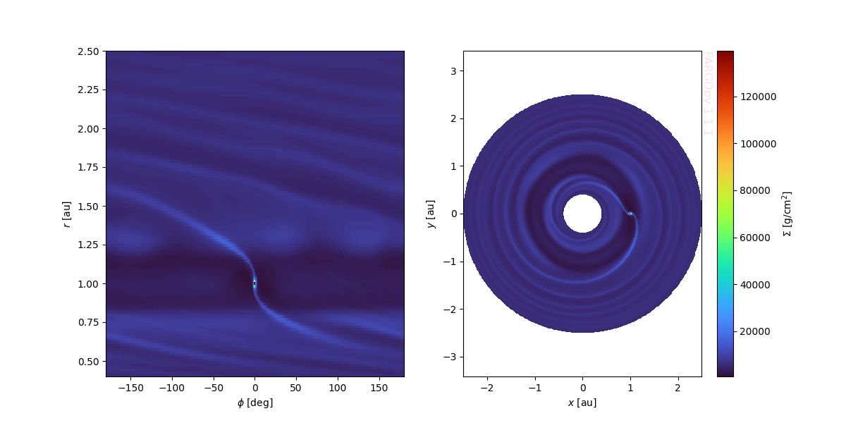
Plot the fields of the FARGO simulation using a colormesh plot:
import matplotlib.pyplot as plt
plt.close('all')
fig,axs = plt.subplots(1,2,figsize=(12,6))
cmap = 'prism_r'

ax = axs[0]
ax.pcolormesh(phi*fp.RAD,r*sim.UL/fp.AU,gasdens_plane*sim.USIGMA,cmap=cmap)
ax.set_xlabel('$\phi$ [deg]')
ax.set_ylabel('$r$ [au]')

ax = axs[1]
c = ax.pcolormesh(x*sim.UL/fp.AU,y*sim.UL/fp.AU,gasdens_plane*sim.USIGMA,cmap=cmap)
ax.set_xlabel('$x$ [au]')
ax.set_ylabel('$y$ [au]')
ax.axis('equal')
fp.Plot.fargopy_mark(ax, frac=1/4)

axc = fig.colorbar(c)
axc.set_label("$\Sigma$ [g/cm$^2$]")
plt.savefig('gallery/fargopy-tutorial-animations_0.png') # Save figure
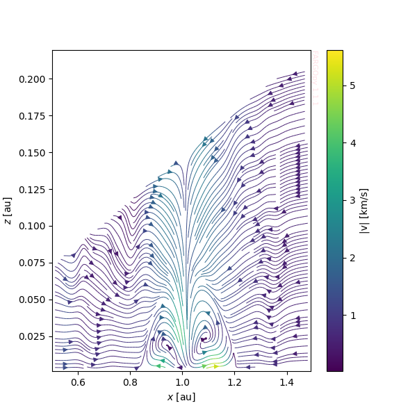
Streamlines
We can visualize the streamlines of the fluid to observe the flow direction at a specific snapshot by interpolating the velocity field. This visualization provides a detailed representation of the velocity field, enabling us to analyze the fluid dynamics and identify key patterns such as vortices, flow separations, or other phenomena of interest. By combining this with contour plots of other fields, such as density or energy, we can gain deeper insights into the interactions and behavior of the simulated system.
We will use the 3D simulation of a disk with a Jovian planet:
fp.Simulation.download_precomputed('p3disoj')
sim = fp.Simulation(output_dir='/tmp/p3disoj')
Downloading p3disoj.tgz from cloud (compressed size around 84 MB) into /tmp

Downloading...
From: https://docs.google.com/uc?export=download&id=1Xzgk9qatZPNX8mLmB58R9NIi_YQUrHz9
To: /tmp/p3disoj.tgz
100%|██████████| 84.2M/84.2M [00:02<00:00, 33.3MB/s]

Uncompressing p3disoj.tgz into /tmp/p3disoj
Done.
Your simulation is now connected with '/local_directory/fargo3d/'
Now you are connected with output directory '/tmp/p3disoj'
Found a variables.par file in '/tmp/p3disoj', loading properties
Loading variables
85 variables loaded
Simulation in 3 dimensions
Loading domain in spherical coordinates:
	Variable phi: 128 [[0, np.float64(-3.117048960983623)], [-1, np.float64(3.117048960983623)]]
	Variable r: 64 [[0, np.float64(0.5078125)], [-1, np.float64(1.4921875)]]
	Variable theta: 32 [[0, np.float64(1.4231400767948967)], [-1, np.float64(1.5684525767948965)]]
Number of snapshots in output directory: 11
Planets found in summary.dat
  Name: Jupiter, Initial pos: [1.0, 0.001, 0.0], Mass: 0.001
First load the density and velocity fields at snapshot 6:
data = sim.load_field(
    fields=['gasv'],
    slice="phi=0",
    snapshot=(0,10)
    )
Now is necesary create a regular mesh where the value of the field is interpolated:
import numpy as np

# This is the snapshot number where the streamplot will be computed
time = 6

# Get the minimum and maximum values of var1 and var3 (x and z coordinates)
xmin=data.var1_mesh[time].min()
xmax=data.var1_mesh[time].max()
zmin=data.var3_mesh[time].min()
zmax=data.var3_mesh[time].max()

# Create a grid of points
resolution = 120
xs = np.linspace(xmin, xmax, resolution)
zs = np.linspace(zmin, zmax, resolution)
X, Z = np.meshgrid(xs, zs, indexing='ij')
Using the mesh we can evaluate the field at any point in space:
vxs, vys, vzs = data.evaluate(field='gasv', time=6, var1=X, var3=Z)

# Velocity magnitude at each mesh point
v_mag = np.sqrt(vxs**2 + vzs**2).T *sim.UV / 1e5
Now we can plot the streamlines of the gas velocity:
fig,axs = plt.subplots(1,1,figsize=(6,6))

cmap = 'Spectral_r'

strm = axs.streamplot(X.T, Z.T, vxs.T, vzs.T,
                       color=v_mag, linewidth=0.7, density=3.0, cmap='viridis')

fig.colorbar(strm.lines, ax=axs, label="|v| [km/s]")

axs.set_xlim(xmin, xmax)
axs.set_ylim(zmin, zmax)
axs.set_xlabel('$x$ [au]')
axs.set_ylabel('$z$ [au]')

fp.Plot.fargopy_mark(axs)
plt.savefig('gallery/readme-streamlines.png') # Save figure
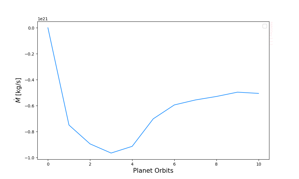
Accretion rate (mass flux)
We compute the mass flux through a closed surface S around the planet. The mass flux (accretion rate) is:\n $$\dot{M}=\int_S\rho(\mathbf{v}\cdot\hat{n}),dS$$ where $\rho$ is the density, $\mathbf{v}$ the velocity vector and $\hat{n}$ the outward normal to the surface. We evaluate this integral by interpolating fields at triangle centers and summing $\rho (\mathbf{v}dotat{n}) A_{i}$ over tessellation triangles.
Define Planet and Surface for Accretion Calculation
Set up the planet and surface objects for the accretion rate calculation.
For this example we will calculate the total flux going through a sphere with a radius equal to the planet's hill radius. For this purpose we need the location and the value of Hill radius of the planet at the snapchot we are interested in:
snap = 10
planet = sim.load_planets(snapshot=snap)[0]
r_hill = planet.hill_radius
print(f"Jupiter Hill Radius: {r_hill * sim.UL / fp.AU:.3f} AU")
Jupiter Hill Radius: 0.068 AU
Now we define the surface over which you want to compute the fluxes:
sphere = fp.Surface(
    type='sphere',
    radius=r_hill,
    subdivisions=3,
)
The computation is performed with follow_planet=True, ensuring that the integration surface co-moves with the planet. This choice is required because the Hill radius evolves in time as a consequence of planetary migration, and therefore the associated control volume must be updated consistently to remain centered on the planet.
acc_rate = sphere.mass_flux(sim=sim, snapshot=[0,snap], follow_planet=True)
Calculating mass flux: 100%|██████████| 11/11 [00:02<00:00, 3.96it/s]
And we can plot it:
snaps = np.linspace(0, snap, len(acc_rate))

fig, ax = plt.subplots(figsize=(10, 6))
ax.plot(snaps, acc_rate * sim.UM / sim.UT, color='dodgerblue')
ax.set_xlabel('Planet Orbits', size=15)
ax.set_ylabel(r'$\dot{M}$ [kg/s]', size=15)
ax.legend(fontsize=12)
fp.Plot.fargopy_mark(ax)
plt.savefig('gallery/readme-accretion.png')
Graphical interface for FARGOpy
In order to ease the manipulation of the FARGO3D data FARGOpy provides a graphical interface written in Python using PyQt5. Below you can find a snapshot of the current version of the interface.
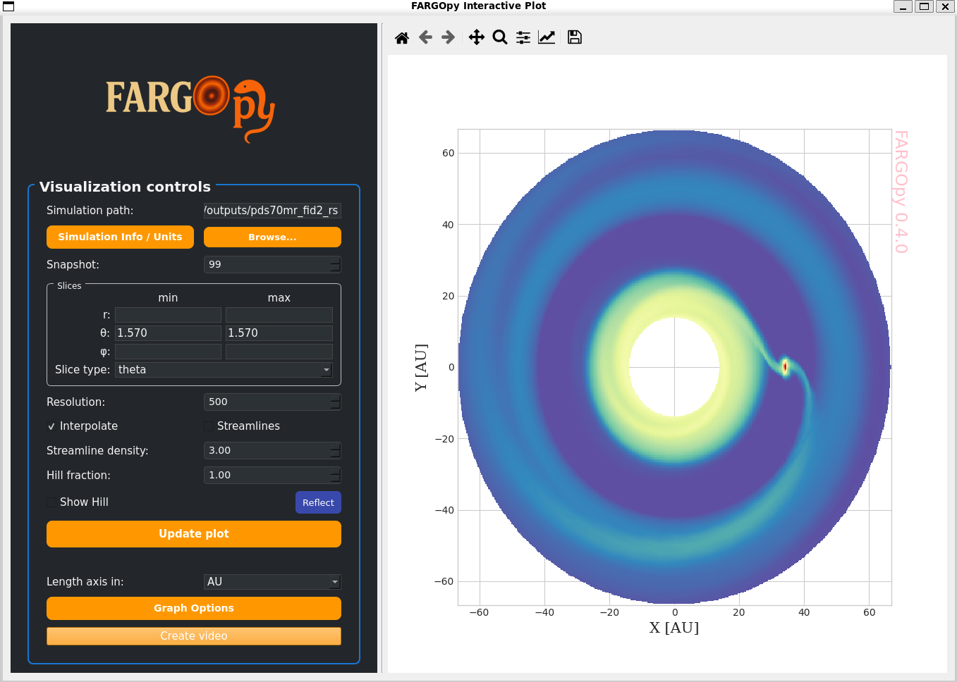
In order to run the graphical interface use:
$ vfargopy
Contributing
We welcome contributions! If you're interested in contributing to MultiNEAs, please:
- Fork the repository
- Create a feature branch
- Make your changes
- Submit a pull request
Please read the CONTRIBUTING.md file for more information.
Citation
If you use FARGOpy in your research, please cite:
@software{fargopy_zenodo_2026,
  author       = {Murillo-Gonzalez, Alejandro and Zuluaga, Jorge I. and Montesinos, Matias},
  title        = {fargopy},
  year         = {2026},
  version      = {1.2.0},
  publisher    = {Zenodo},
  doi          = {10.5281/zenodo.19430858},
  url          = {https://doi.org/10.5281/zenodo.19430858},
  note         = {Concept DOI: 10.5281/zenodo.19430857}
}

@misc{MurilloGonzalezZuluagaMontesinos2026,
  author        = {Murillo-Gonzalez, Alejandro and Zuluaga, Jorge I. and Montesinos, Matias},
  title         = {Three-dimensional circumplanetary flows in a PDS 70c-inspired system: hydrodynamic simulations with FARGO3D and analysis with FARGOpy},
  year          = {2026},
  eprint        = {0000.00000},
  archivePrefix = {arXiv},
  primaryClass  = {astro-ph.EP},
  url           = {https://arxiv.org/abs/0000.00000}
}

@misc{MurilloGonzalez2026,
  author       = {Murillo-Gonzalez, Alejandro and Zuluaga, Jorge I. and Montesinos, Matias},
  title        = {{FARGOpy}: A {Python} Package for Post-processing and Analyzing {FARGO3D} Hydrodynamical Simulations},
  year         = {2026},
  howpublished = {\url{https://github.com/seap-udea/fargopy/blob/main/science/introducing-fargopy/MurilloZuluagaMontesinos2026-IntroducingFARGOpy.pdf}},
  note         = {Manuscript hosted on GitHub}
}
Replace 0000.00000 once the arXiv identifier is assigned.
Project details
Release history Release notifications | RSS feed


Download files
Download the file for your platform. If you're not sure which to choose, learn more about installing packages.
Source Distribution
Built Distribution
Filter files by name, interpreter, ABI, and platform.
If you're not sure about the file name format, learn more about wheel file names.
Copy a direct link to the current filters
File details
Details for the file fargopy-1.2.1.tar.gz.
File metadata
- Download URL: fargopy-1.2.1.tar.gz
- Upload date:
- Size: 2.3 MB
- Tags: Source
- Uploaded using Trusted Publishing? No
- Uploaded via: twine/6.2.0 CPython/3.12.5
File hashes
| Algorithm | Hash digest | |
|---|---|---|
| SHA256 |
a2f82fc57f5829b49247b8d2cc5bfbec2e800d86250fcf7d1b3f04b0e9e9821d
|
|
| MD5 |
a14d17573bc6c813a4df680329913d13
|
|
| BLAKE2b-256 |
87790f980b048d09b1f68cf0512f7909e981f87c189ab6df4ea6407bcc4cc06e
|
File details
Details for the file fargopy-1.2.1-py3-none-any.whl.
File metadata
- Download URL: fargopy-1.2.1-py3-none-any.whl
- Upload date:
- Size: 2.3 MB
- Tags: Python 3
- Uploaded using Trusted Publishing? No
- Uploaded via: twine/6.2.0 CPython/3.12.5
File hashes
| Algorithm | Hash digest | |
|---|---|---|
| SHA256 |
6bc3bcd89a268893864ddb44b6de6f77d2f1578d3dbb8693d6e6f155379c537a
|
|
| MD5 |
2663243ebdaff1f2997b316ea16237fe
|
|
| BLAKE2b-256 |
444aba46a4564a654aba13dc08c0e28d36020373995866444cbf21dc1772a5a1
|


