Financial Time Series Plotting Libarary

Project description
FinTime
FinTime is a financial time series plotting library built on Matplotlib.
Features:
- Visual elements as standalone objects (Artists).
- Dynamically sized composite structures (Grid, Subplots, Panels) organise multiple plots within a figure.
- Branched propagation of data and configurations to sub-components, enabling overrides at any level.
Table of Contents
Installation
pip install fintime
The Plot Function
Before delving into the inner workings of the plot function, let's briefly introduce the key concepts that help organize your figure.
Terminology
- Artist: An object capable of drawing a visual on an Axes.
- Panel: Panels serve as the canvas for either one Axes or two twinx Axes.
- Subplot: A collection of panels is referred to as a Subplot. Panels within a Subplot are visually stacked vertically and share the x-axis.
- Grid: A collection of Subplots. This object is not exposed directly but manages its Subplots.
Flow
The flow of the plot function unfolds in the following sequential steps:
-
Initialization: When subplots are provided, a
Gridobject is populated. Alternatively, if panels are passed, aSubplotobject functions as the top-level container, resulting in a hierarchical structure:grid -> subplots -> panels -> artists.subplot -> panels -> artists
-
Config and Data Propagation: Configurations and data flow down the hierarchical structure, enabling components to incorporate local changes received during instantiation. Fintime's configuration object (
fieldconfig.Config) ensures the correctness of configuration settings, triggering exceptions for any invalid values. -
Data Validation: Following the merging of data and configurations across components, a data validation step ensures that all components are prepared for successful rendering later on.
-
Component Sizing: The sizing of components is intricately tied to the hierarchical structure. While artists can employ dynamic sizing with best-effort defaults, each component provides a
sizeargument, granting it precedence over any dynamic settings. Sizing information is propagated upward in the hierarchical structure, and whenever fixed sizing is specified, it takes precedence. In such cases, the dimensions of components are determined based on their size ratios. -
Finalize Sizing: Conclusive sizing information is computed and cascaded down through the components, communicating their final dimensions. This information is used to enhance the final appearance of the plot, influencing aspects like tick densities, line widths, and more.
-
Drawing: In the final stage, cascading down the hierarchical structure once more, each container invokes the
drawmethod of its components, instantiating actual Matplotlib objects along the way. Artists then draw onto Axes, completing the visualization process.
Usage
Data
FinTime expects data to be structured as a flat mapping, such as a dictionary, containing NumPy arrays. The example below demonstrates the generation of mock OHLCV data with intervals of 1, 10, 30, and 300 seconds. This data will be used in the following examples.
from fintime.mock.data import (
    generate_random_trade_ticks,
    add_random_trades,
    add_random_imb,
    add_moving_average,
)
from fintime.mock.data import to_timebar

spans = [1, 10, 30, 300]
ticks = generate_random_trade_ticks(seed=1)
datas = {f"{span}s": to_timebar(ticks, span=span) for span in spans}

for span in spans:
    data = datas[f"{span}s"]
    add_random_imb(data)
    add_random_trades(data, 10)
    add_moving_average(data, 20)

for feat, array in datas["10s"].items():
    print(feat.ljust(6), repr(array[:2]))

# --> dt     array(['2024-03-18T16:43:10.000', '2024-03-18T16:43:20.000'], dtype='datetime64[ms]')
# --> open   array([101.61, 101.61])
# --> high   array([101.76, 101.92])
# --> low    array([101.54, 101.57])
# --> close  array([101.61, 101.57])
# --> vol    array([2824, 2749])
# --> imb    array([ 0.41030182, -0.44632449])
# --> price  array([0., 0.])
# --> side   array([None, None], dtype=object)
# --> size   array([0., 0.])
# --> ma20   array([nan, nan])
Panels Plot
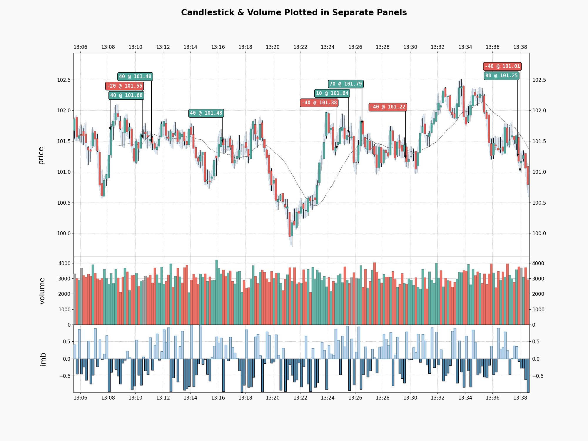
Let's proceed and plot candlesticks and volume bars with a 10-second span.
from matplotlib.pylab import plt
from fintime.plot import plot, Panel
from fintime.artists import (
    CandleStick,
    Volume,
    DivergingBar,
    FillBetween,
    TradeAnnotation,
    Line,
)


fig = plot(
    specs=[
        Panel(
            artists=[
                CandleStick(),
                FillBetween(y1_feat="low", y2_feat="high"),
                TradeAnnotation(),
                Line(yfeat="ma20"),
            ]
        ),
        Panel(artists=[Volume()]),
        Panel(artists=[DivergingBar(feat="imb")]),
    ],
    data=datas["10s"],
    title="Candlestick & Volume Plotted in Separate Panels",
)
plt.show()
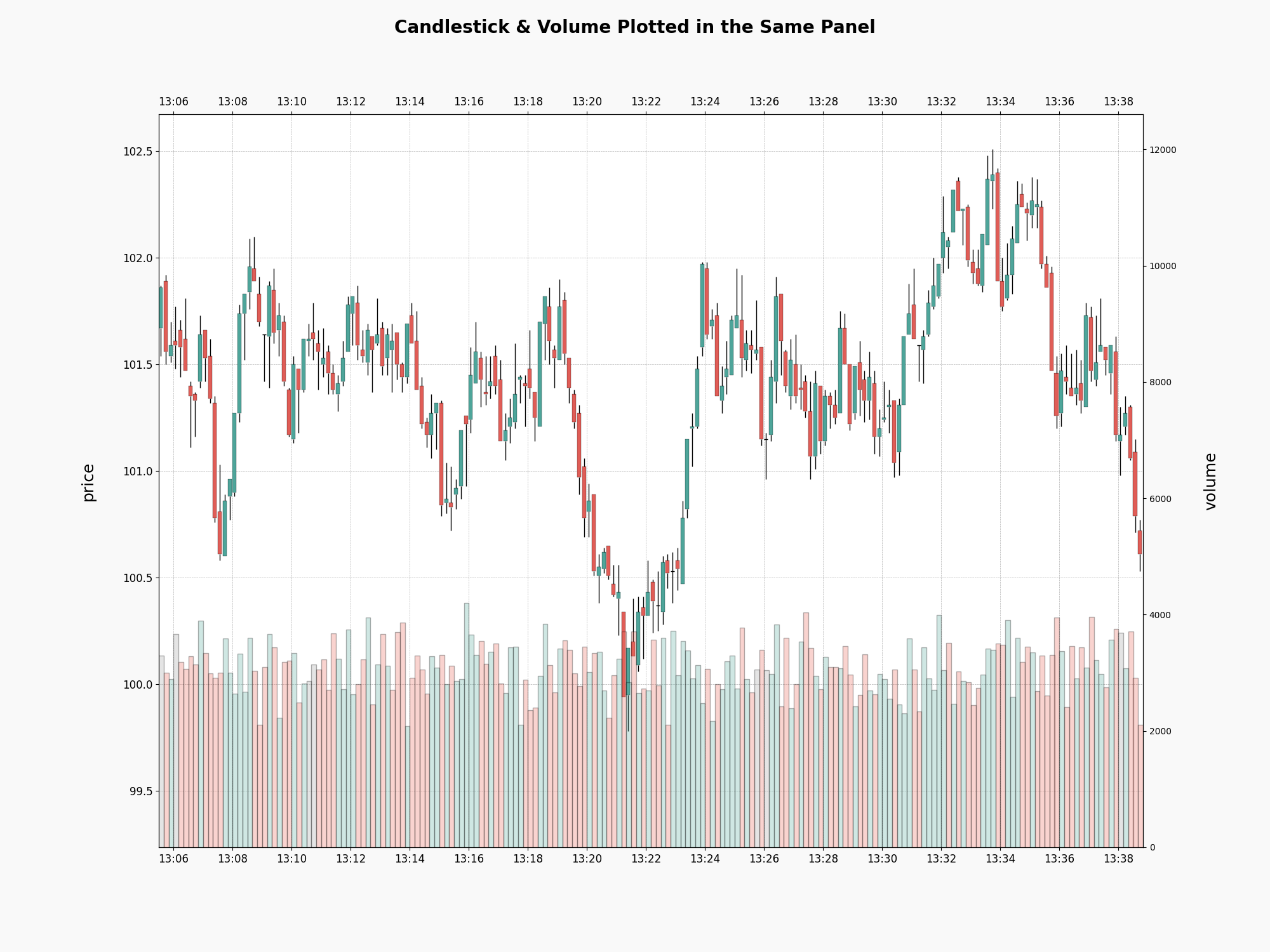
Alternatively, it is also possible to draw Candlesticks and Volumebars in the same panel.
fig = plot(
    specs=[
        Panel(
            artists=[
                CandleStick(config={"candlestick.padding.ymin": 0.2}),
                Volume(
                    twinx=True,
                    config={
                        "volume.edge.linewidth": 1,
                        "volume.face.alpha": 0.3,
                        "volume.edge.alpha": 0.5,
                        "volume.padding.ymax": 2,
                        "volume.relwidth": 1,
                    },
                ),
            ]
        ),
    ],
    data=datas["10s"],
    figsize=(20, 15),
    title="Candlestick & Volume Plotted in the Same Panel",
)
plt.show()
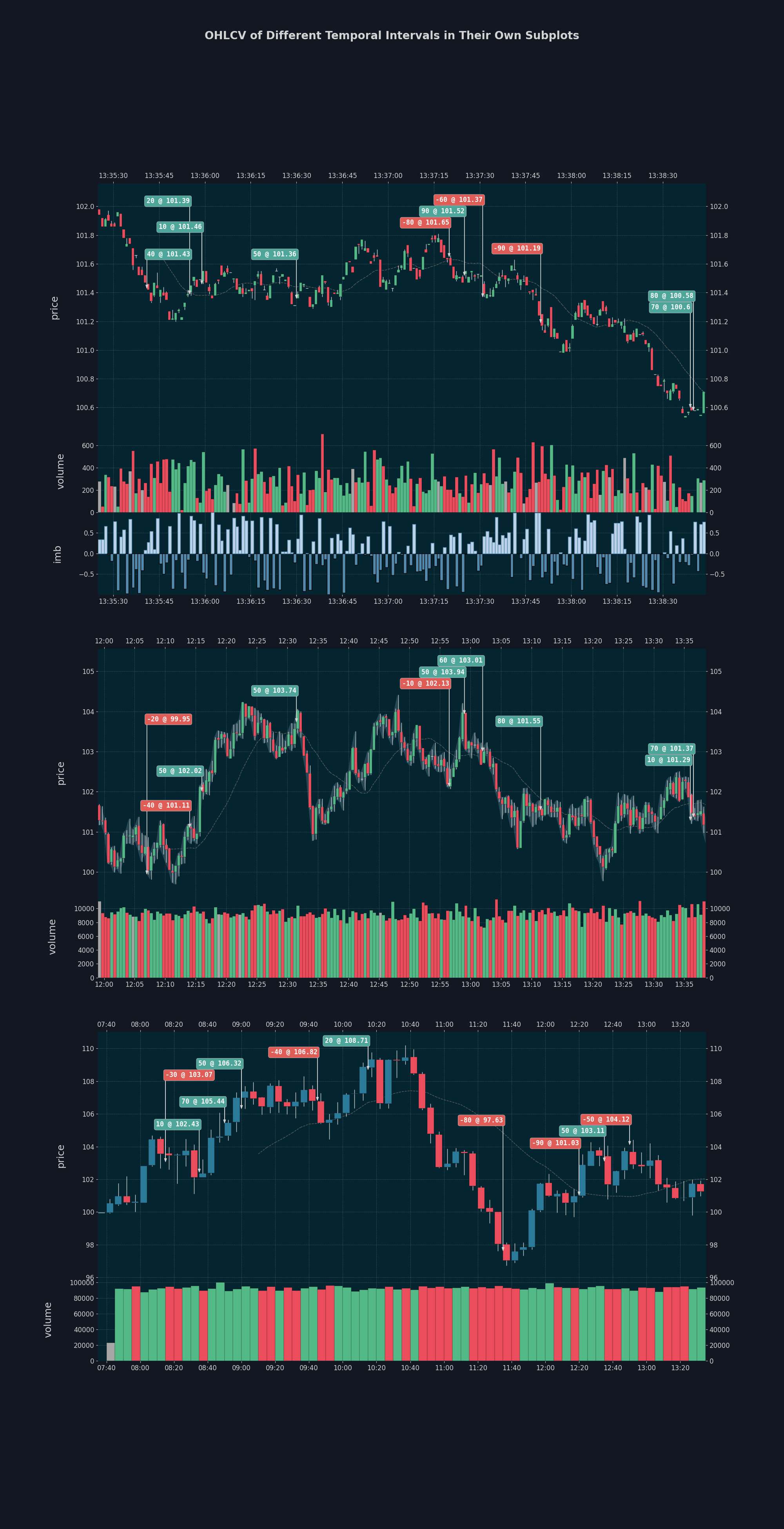
Subplots Plot
Displaying multiple groups of panels within a single figure is achieved by passing a list of Subplots (rather than Panels) to the plot function. In the following example, we will draw candlestick and volume bars with spans of 1, 30 and 300 seconds while overriding some configurations.
from fintime.plot import Subplot
from fintime.config import get_config

config = get_config()
config.figure.facecolor = "#131722"
config.figure.title.color = "lightgray"
config.panel.facecolor = "#042530"
config.panel.spine.color = config.panel.facecolor
config.grid.color = "lightgray"
config.xlabel.color = "lightgray"
config.ylabel.color = "lightgray"
config.candlestick.body.face.color.up = "#53b987"
config.candlestick.body.face.color.down = "#eb4d5c"
config.candlestick.wick.color = "lightgray"
config.candlestick.doji.color = "lightgray"
config.volume.face.color.up = "#53b987"
config.volume.face.color.down = "#eb4d5c"
config.fill_between.alpha = 0.2
config.trade_annotation.text.bbox.edge.linewidth = 0.5
for side in ["buy", "sell"]:
    config.trade_annotation.arrow.edge.color[side] = "lightgray"
    config.trade_annotation.arrow.face.color[side] = "lightgray"
    config.trade_annotation.text.bbox.edge.color[side] = "lightgray"


subplots = [
    Subplot(
        [
            Panel(
                artists=[
                    CandleStick(data=datas["1s"]),
                    TradeAnnotation(data=datas["1s"]),
                    Line(data=datas["1s"], yfeat="ma20"),
                ]
            ),
            Panel(artists=[Volume(data=datas["1s"])]),
            Panel(artists=[DivergingBar(data=datas["1s"], feat="imb")]),
        ]
    ),
    Subplot(
        [
            Panel(
                artists=[
                    TradeAnnotation(),
                    CandleStick(),
                    Line(yfeat="ma20"),
                    FillBetween(y1_feat="low", y2_feat="high"),
                ]
            ),
            Panel(artists=[Volume()]),
        ],
        data=datas["30s"],
    ),
    Subplot(
        [
            Panel(
                artists=[
                    CandleStick(
                        config={"candlestick.body.face.color.up": "#2c7a99"}
                    ),
                    TradeAnnotation(),
                    Line(yfeat="ma20"),
                ]
            ),
            Panel(artists=[Volume()]),
        ],
        data=datas["300s"],
    ),
]

fig = plot(
    subplots,
    title="OHLCV of Different Temporal Intervals in Their Own Subplots",
    config=config,
)
plt.show()
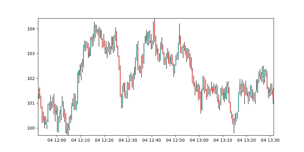
Standalone Use of Artists
You also have the option to have Artists draw on your own Axes.
import matplotlib.pyplot as plt
from fintime.config import get_config

data = datas["30s"]
fig = plt.Figure(figsize=(10, 5))
axes = fig.subplots()
axes.set_xlim(min(data["dt"]), max(data["dt"]))
axes.set_ylim(min(data["low"]), max(data["high"]))

cs_artist = CandleStick(data=data, config=get_config())
cs_artist.draw(axes)
plt.show()
Configuration
FinTime provides granular control over configurations through its config argument, available in the plot function, subplot, panel, and artists classes. These configurations are propagated downward to sub-components, including updates along each branch.
FinTime uses FieldConfig for configurations, and, as demonstrated in the examples it supports updates by passing a new Config object or a dictionary, whether flat or nested. If you're interested in creating your own configurations, please refer to the documentation.
The available configuration options can be displayed using:
from fintime.config import get_config

cfg = get_config()
for k, v in cfg.to_flat_dict().items():
    print(k.ljust(30), v)

# Expected output:
# --> font.family                    sans-serif
# --> font.color                     black
# --> font.weight                    300
# --> ylabel.font.family             sans-serif
# --> ylabel.font.color              black
# --> ylabel.font.weight             300
# --> ylabel.font.size               18
# --> ylabel.pad                     30
# --> ...
Upcoming Features
- Legends
- Custom y-tick formatting
- Improved default spacing logic
- Support for non-linear datetime xaxis to display OHCV data of irregular intervals
- More artists:
- Trading session shading
- Table
- and more
Note of Warning
FinTime is currently in its early alpha development stage, and interfaces are subject to change without prior notice, including potential modifications that may not be backward compatible. Please be aware of this ongoing development state.


Download files
Download the file for your platform. If you're not sure which to choose, learn more about installing packages.
Source Distribution
Built Distribution
Filter files by name, interpreter, ABI, and platform.
If you're not sure about the file name format, learn more about wheel file names.
Copy a direct link to the current filters
File details
Details for the file fintime-0.1.6.tar.gz.
File metadata
- Download URL: fintime-0.1.6.tar.gz
- Upload date:
- Size: 22.4 kB
- Tags: Source
- Uploaded using Trusted Publishing? No
- Uploaded via: poetry/1.8.2 CPython/3.12.2 Linux/6.5.0-35-generic
File hashes
| Algorithm | Hash digest | |
|---|---|---|
| SHA256 |
ea8d920be015c086352cdc3ba33c710d8fc7760e7dd2279cedcb990b05aa41f7
|
|
| MD5 |
edcec5ea1500c7be090744ad8051d146
|
|
| BLAKE2b-256 |
cc91d4c6616e02bfff98e967b4582faea75cef532ad8549c19335ed3b0aea0c9
|
File details
Details for the file fintime-0.1.6-py3-none-any.whl.
File metadata
- Download URL: fintime-0.1.6-py3-none-any.whl
- Upload date:
- Size: 24.9 kB
- Tags: Python 3
- Uploaded using Trusted Publishing? No
- Uploaded via: poetry/1.8.2 CPython/3.12.2 Linux/6.5.0-35-generic
File hashes
| Algorithm | Hash digest | |
|---|---|---|
| SHA256 |
94e69df59794db6a04a7880f7fb541429e1a43a9b9dc2417e464eed080f72e1a
|
|
| MD5 |
fa35811685b0048913300e04ade4388d
|
|
| BLAKE2b-256 |
2e7ffc0a007b1317d3cd304678f0e070c7eb4405c8b87409c8e6718b4fe53d37
|


