
FlashDeconv





Estimate spatial cell-type proportions at atlas scale.
FlashDeconv estimates cell type proportions from spatial transcriptomics data (Visium, Visium HD, Stereo-seq). It is designed for large-scale analyses where computational efficiency is essential, using reference-derived gene weighting and sparse spatial regularization.
Paper: Yang, C., Zhang, X. & Chen, J. FlashDeconv enables atlas-scale, multi-resolution spatial deconvolution via structure-preserving sketching. bioRxiv (2025). DOI: 10.64898/2025.12.22.696108
Installation
pip install "flashdeconv[io,scanpy]"
Requires Python 3.9–3.14. This installs the dependencies used in the Quick Start below. For development or additional I/O support, see Installation Options.
Quick Start
import scanpy as sc
import flashdeconv as fd

# Load count matrices, spatial coordinates, and reference cell-type labels
adata_st = sc.read_h5ad("spatial.h5ad")
adata_ref = sc.read_h5ad("reference.h5ad")

# Deconvolve
fd.tl.deconvolve(adata_st, adata_ref, cell_type_key="cell_type")

# Rows are spatial locations; columns are reference cell types
proportions = adata_st.obsm["flashdeconv"]
print(proportions.head())
The example expects raw counts in .X, spatial coordinates in adata_st.obsm["spatial"], and reference labels in adata_ref.obs["cell_type"]. If counts are stored in layers, pass layer_st="counts" and layer_ref="counts". Match gene identifiers across datasets before running; the AnnData interface intersects and aligns shared genes.
FlashDeconv is also available as a tool in ChatSpatial, an MCP server for spatial transcriptomics — run deconvolution through natural language from any compatible client.
How it works
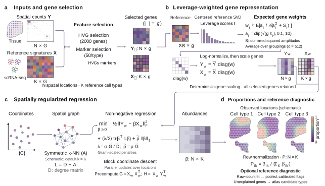
- Select the union of spatial highly variable genes and reference markers; derive leverage scores from the reference signatures.
- Apply the selected preprocessing (by default
log1pof expression normalized to 10,000 counts per spot or cell type) and a shared deterministic leverage-weighted gene representation to spatial and reference expression: each selected gene is scaled by its exact expected weight in a column-normalized leverage-weighted CountSketch withsketch_dimbuckets (default 512), averaged analytically over the random bucket assignment. No random projection is drawn, so results do not depend onrandom_state. The previous randomized CountSketch projection (uniform hashing, random signs, leverage-weighted amplitudes) remains available withgene_weighting="countsketch". - Construct a sparse spatial neighbor graph and fit non-negative regression coefficients with spatial smoothing and an L1 penalty.
- Normalize each coefficient row to obtain estimated cell-type proportions.
The regression operates on the weighted (or, in legacy mode, sketched) matrices:
minimize ½‖Y_s − βX_s‖²_F + ½λ Tr(βᵀLβ) + ρ_eff‖β‖₁, subject to β ≥ 0
Here Y_s is N × p and X_s is K × p, with p the number of selected genes (p = sketch_dim in legacy mode), and L = D − A is the spatial graph Laplacian. The solver scales the user parameter as ρ_eff = rho_sparsity × mean(diag(X_s X_sᵀ)).
beta_ contains regression coefficients, not absolute cell counts. proportions_ contains their row-normalized values, P[i, k] = β[i, k] / sum(β[i, :]). An all-zero coefficient row is assigned a uniform distribution as a numerical fallback, not evidence of equal biological composition.
With fixed gene count, cell-type count, iteration count, and bounded graph degree, the regression stage has linear time and memory scaling in the number of spots. End-to-end runtime also includes preprocessing and neighbor search; it is not an unconditional O(N) guarantee. Radius graphs can become dense when many spots fall within the radius.
Performance
Scalability
| Spots | Time | Memory |
|---|---|---|
| 10,000 | < 1 sec | < 1 GB |
| 100,000 | ~4 sec | ~2 GB |
| 1,000,000 | ~3 min | ~21 GB |
Reported on MacBook Pro M2 Max (32GB unified memory), CPU-only. The million-spot result uses simulated data. These timings describe the benchmark configurations, not a runtime guarantee for arbitrary gene counts, cell-type counts, or graph settings.
Accuracy
On the 54 Silver Standard datasets (6 tissues × 9 abundance patterns) from the Spotless benchmark:
| Metric | FlashDeconv | RCTD | Cell2Location |
|---|---|---|---|
| Mean Pearson correlation | 0.944 | 0.934 | 0.918 |
Values follow the current manuscript’s unified benchmark table (Silver Standard rows). These datasets use simulated mixtures; rankings differ on real-data benchmarks. See the reproducibility repository for benchmark materials. Evaluate performance on data and reference conditions relevant to your application.
API
See the Quick Start for the AnnData interface and the full API reference for methods, I/O utilities, and evaluation functions.
NumPy
Provide spatial counts Y (N × G, dense or SciPy sparse), reference signatures X (K × G), and coordinates coords (N × 2 or N × 3). The columns of Y and X must contain the same genes in the same order, and both must be non-negative and finite.
from flashdeconv import FlashDeconv

model = FlashDeconv(
    sketch_dim=512,
    lambda_spatial="auto",
    n_hvg=2000,
    k_neighbors=6,
    random_state=0,
)
proportions = model.fit_transform(Y, X, coords)
Parameters
| Parameter | Default | Description |
|---|---|---|
gene_weighting |
"expected" | Gene representation: "expected" (deterministic expected leverage-weighted CountSketch weights) or "countsketch" (legacy randomized projection) |
sketch_dim |
512 | CountSketch bucket count d (sets the expected weights; projection dimension in legacy mode) |
lambda_spatial |
"auto" | Spatial regularization, automatically scaled by default |
rho_sparsity |
0.01 | L1 sparsity penalty (dimensionless fraction) |
n_hvg |
2000 | Highly variable genes |
n_markers_per_type |
50 | Marker genes per cell type |
spatial_method |
"knn" | Graph method: "knn", "radius", or "grid" |
k_neighbors |
6 | Spatial graph neighbors (for "knn") |
radius |
None | Neighbor radius (required for "radius") |
max_iter |
1000 | Maximum solver iterations |
tol |
1e-4 | Convergence tolerance (relative change of the coefficients) |
preprocess |
"log_cpm" | Normalization: "log_cpm" (log1p of counts per 10,000), "pearson", or "raw" |
random_state |
0 | Random seed for the legacy CountSketch projection (unused by the default) |
Output
| Attribute | Description |
|---|---|
proportions_ |
Cell type proportions (N × K), sum to 1 |
beta_ |
Unnormalized regression coefficients (N × K) |
info_ |
Convergence statistics |
Input Formats
- Spatial data: AnnData, NumPy array (N × G), or SciPy sparse matrix
- Reference: AnnData (aggregated by cell type) or NumPy array (K × G)
- Coordinates: Extracted from
adata.obsm["spatial"]or NumPy array (N × 2 or N × 3)
Reference quality and limitations
- Use reference annotations supported by marker expression, and check that expected tissue cell types are represented. Missing types can distort the estimated proportions of included types.
- Assess signature stability across cells or donors. Required sample size depends on heterogeneity, sequencing depth, and separation between types; there is no universal cell-count or marker-fold-change cutoff.
- Inspect highly correlated signatures and consider a coarser annotation when subtypes cannot be distinguished reliably.
- Review labels such as
UnknownorUnassignedbefore aggregation. A heterogeneous pool can produce an ambiguous signature, but the label alone is not a reason to discard a coherent population. - Spatial smoothing can blur sharp boundaries. Compare smoothing strengths when boundaries or rare populations are central to the analysis.
- Estimated proportions depend on reference quality and preprocessing; they are not direct measurements of cell numbers. The opt-in uncertainty estimates (
compute_uncertainty,bootstrap_uncertainty) are model-based: they reflect sampling uncertainty under the fitted model and exclude reference–tissue mismatch, missing cell types and model misspecification, which usually dominate the error. Use them to compare estimate stability across spots and types, not as calibrated intervals for true proportions.
Installation Options
# Standard
pip install flashdeconv

# With AnnData support
pip install "flashdeconv[io]"

# Development
git clone https://github.com/cafferychen777/flashdeconv.git
cd flashdeconv && pip install -e ".[dev]"
Requirements: Python 3.9–3.14, numpy, scipy, numba. Optional: scanpy, anndata.
Citation
If you use FlashDeconv in your research, please cite:
Yang, C., Zhang, X. & Chen, J. FlashDeconv enables atlas-scale, multi-resolution spatial deconvolution via structure-preserving sketching. bioRxiv (2025). DOI: 10.64898/2025.12.22.696108
@article{yang2025flashdeconv,
  title={FlashDeconv enables atlas-scale, multi-resolution spatial deconvolution
         via structure-preserving sketching},
  author={Yang, Chen and Zhang, Xianyang and Chen, Jun},
  journal={bioRxiv},
  year={2025},
  doi={10.64898/2025.12.22.696108}
}
Resources
- Paper reproducibility code
- Stereo-seq guide — Platform-specific considerations
- GitHub Issues
- BSD-3-Clause License
Acknowledgments
We thank the developers of Spotless, Cell2Location, RCTD, CARD, and other deconvolution methods whose work contributed to this field.
1 maintainer

Metadata
1 maintainer
Release files for flashdeconv 0.2.0
For a detailed explanation of source distributions (sdists) and built distributions (wheels), please see the package formats documentation.
Source distribution (sdist)
| File | Size | Uploaded | |
|---|---|---|---|
| flashdeconv-0.2.0.tar.gz | 73.7 kB | Details |
Built distribution (wheel)
| File | Interpreter | ABI | Platform | Reset |
|---|---|---|---|---|
| flashdeconv-0.2.0-py3-none-any.whl | Python 3 | none | any | Details |
Total release size: 134.4 kB
Release files / flashdeconv-0.2.0.tar.gz
| Download URL | flashdeconv-0.2.0.tar.gz |
|---|---|
| Size | 73.7 kB |
| Tags | Source |
|
SHA-256 checksum How to use checksums |
5817bfdfe97298f7a647d32524422c10cc17faeb20af4d1c43508a84f6980c3e
|
|
BLAKE2b-256 checksum How to use checksums |
f563f1b81572d65cb012f6475731f2ebd787978c2d335e81a0a96338bbcea42b
|
| Upload date | |
|
Uploaded using Trusted Publishing? What is trusted publishing? |
Yes |
| Uploaded via |
twine/7.0.0 CPython/3.13.14
|
Provenance
Provenance describes where a file came from. On PyPI, provenance is shared via attestations, which provide a verifiable record of the build or publishing details. View details, limitations and caveats.


PyPI Publish Attestation
PyPI verified that this artifact, at this checksum, originated from the publisher listed below.
Signed by GitHub Actions, verified by PyPI on Sep 28, 2026.
Transparency logRelease files / flashdeconv-0.2.0-py3-none-any.whl
| Download URL | flashdeconv-0.2.0-py3-none-any.whl |
|---|---|
| Size | 60.7 kB |
| Tags | Python 3 |
|
SHA-256 checksum How to use checksums |
157a12c678af883207a037bcf075a58ae6b26e8a0529ff7601416a62ea4bb55d
|
|
BLAKE2b-256 checksum How to use checksums |
6b05c03aaad3e0eef625e6ec1e6b2f17e164ce4a41bcd157626ad1035a50dc21
|
| Upload date | |
|
Uploaded using Trusted Publishing? What is trusted publishing? |
Yes |
| Uploaded via |
twine/7.0.0 CPython/3.13.14
|
Provenance
Provenance describes where a file came from. On PyPI, provenance is shared via attestations, which provide a verifiable record of the build or publishing details. View details, limitations and caveats.
PyPI Publish Attestation
PyPI verified that this artifact, at this checksum, originated from the publisher listed below.
Signed by GitHub Actions, verified by PyPI on Sep 28, 2026.
Transparency log













