
fxtensor-bayesnet
English | 日本語
A config-driven inference tool for discrete Bayesian networks, built on fxtensor-salmon.
Overview
fxtensor-bayesnet is a decision-support tool that expresses cause-and-effect relationships between events as conditional probabilities and quantifies their overall impact. Assumptions and probabilities live in a configuration file, so they can be revised quickly without changing any code. It supports comparing multiple scenarios as well as working backwards from observed outcomes to their likely causes. Because the configuration and results can be recorded daily, the rationale behind each judgement and how it changed over time can be tracked continuously.
How it works:
- Each variable is discrete and takes one of a finite set of labels (e.g.
Clear / Cloudy / Overcast). - Variables without parents (roots) get a prior distribution; child variables get a conditional probability table ("parent label combination → child distribution", i.e. a Markov kernel).
- The joint distribution is built by composing states and kernels with fxtensor-salmon's
FXTensor. From it the tool computes marginals per scenario, conditioning on observations (Bayesian updating), and root-cause inference viabayesian_inversion. - On every run, results computed with the library are cross-checked against a direct numpy
einsumcomputation, using unrounded values; any mismatch stops the run (see the検算("checks") field of the results). - When the joint distribution would exceed 2 million entries, the tool automatically switches to computing over ancestor sets only (same results). Conditioning never builds a dense wiring kernel larger than 1 million entries; above that it sums the joint directly or uses variable elimination.
- Causal questions (0.10.0):
interventionsapply do() to any variable (root or not) by graph surgery, andeffectsreport the average causal effect (ACE) next to the observational difference, so confounding becomes visible. - Observations can combine several pieces of evidence and soft (likelihood) evidence;
sensitivityranks the prior / CPT entries a result depends on most. --plotrenders the network structure, scenario comparison, Bayesian updates and day-over-day changes as PNG / SVG (requires matplotlib).
The probabilities in a config are the user's assumptions. The results are consequences of those assumptions; the tool does not validate the assumptions themselves.
Installation
Python 3.8 or later. Install from PyPI:
pip install fxtensor-bayesnet            # core (pulls in numpy and fxtensor-salmon)
pip install "fxtensor-bayesnet[plot]"    # with figures (adds matplotlib)
For development:
git clone https://github.com/salmonsnare/fxtensor-bayesnet.git
cd fxtensor-bayesnet
python3 -m venv .venv
. .venv/bin/activate
pip install -e ".[dev]"     # includes pytest and matplotlib
pytest
Quick start
Example configs live in examples/ (they are not part of the PyPI package, so fetch them from the repository).
curl -o config.json https://raw.githubusercontent.com/salmonsnare/fxtensor-bayesnet/v0.10.0/examples/weather/config.en.json
fxtensor-bayesnet --check                            # defaults to ./config.json
fxtensor-bayesnet --no-write --md --lang en          # Markdown to stdout
fxtensor-bayesnet --no-write --plot --lang en --out-dir out/   # figures only, into out/
# python -m fxtensor_bayesnet ... works the same way
Writing a config
A config is a single JSON file. Minimal example:
{
  "as_of": "2026-10-10",
  "horizon": "Next day",
  "note": "All probabilities are assumptions",
  "variables": {
    "cloud": {"name": "Cloud cover", "labels": ["Clear", "Cloudy"]},
    "rain":  {"name": "Precipitation", "labels": ["None", "Some"]}
  },
  "priors": {
    "cloud": {"p": [0.6, 0.4], "reason": "free-text rationale (optional)"}
  },
  "kernels": {
    "rain": {
      "parents": ["cloud"],
      "reason": "free-text rationale (optional)",
      "cpt": {
        "Clear": [0.95, 0.05],
        "Cloudy": [0.6, 0.4]
      }
    }
  },
  "scenarios": {
    "A: Mostly cloudy": {"cloud": [0.2, 0.8]}
  },
  "observations": [
    {"var": "rain", "label": "Some", "focus": ["cloud"]}
  ],
  "outputs": ["rain"]
}
| Key | Required | Meaning |
|---|---|---|
as_of |
yes | Reference date (YYYY-MM-DD); used as the snapshot folder name |
horizon / note |
Forecast horizon and a note (shown in the results) | |
variables |
yes | Variable → {"name": display name, "labels": [labels…]}. At least 2 labels, no duplicates |
priors |
yes | Root variable → {"p": [probability per label], "reason": optional}. Must sum to 1 |
kernels |
yes | Child variable → {"parents": [parents…], "cpt": {...}, "reason": optional} |
scenarios |
Scenario name → {root variable: replacement prior}. A base scenario is always included |
|
observations |
{"var", "label", "focus"}. Computes posteriors given var=label. For the focus variables it also reports prior→posterior movement (difference, total variation distance TV, KL) and ranks them by movement (defaults to all roots). Instead of var/label, {"evidence": {...}, "name": optional} conditions on several observations jointly and accepts soft evidence (see below) |
|
interventions |
Name → {variable: label or [distribution]}. do() on any variable by graph surgery (its kernel is replaced); reports the marginals of outputs |
|
effects |
List of {"treatment", "outcome", "outcome_label"?, "treated"?, "control"?}. P(outcome | do(X=x)) and P(outcome | X=x) for every level, the ACE (treated − control), the observational difference and their gap. Defaults: last label of the outcome, treated = last label, control = first label |
|
sensitivity |
{"target", "label"?, "delta"? (0.05), "top"? (10)} or a list of them. One-at-a-time sensitivity of P(target=label) to every prior and CPT entry |
|
outputs |
Variables shown in the result tables (defaults to all non-root variables) |
Writing a cpt:
- Each key joins the parents' labels with
|, inparentsorder (e.g. with parents["load", "age"]:"High|Old"). - Each value lists probabilities in the child's label order; every row must sum to 1.
- Every combination of parent labels needs a row (missing or extra rows are reported by
--check). - Each variable goes in exactly one of
priorsorkernels. No cycles. Up to 52 variables. - Variables may be declared in any order in
variables(roots do not have to come first).
Interventions, causal effects, evidence and sensitivity
These keys are optional; configs without them give exactly the same results as before. Example additions to the maintenance example (examples/maintenance/config.en.json):
"interventions": {
  "Replace worn parts (wear=Low)": {"wear": "Low"},
  "Cool half of the bearings": {"temp": [0.5, 0.5]}
},
"effects": [
  {"treatment": "temp", "outcome": "failure", "outcome_label": "Shutdown"},
  {"treatment": "wear", "outcome": "failure", "outcome_label": "Shutdown", "treated": "High", "control": "Low"}
],
"observations": [
  {"evidence": {"vibration": "Abnormal", "temp": "Elevated"}, "focus": ["load", "age", "service"]},
  {"name": "Vibration probably abnormal (noisy sensor)",
   "evidence": {"vibration": {"likelihood": [0.1, 0.4, 0.9]}}, "focus": ["wear"]}
],
"sensitivity": {"target": "failure", "label": "Shutdown", "delta": 0.05, "top": 5}
interventions:{"wear": "Low"}is a hard do(wear=Low); a list such as[0.5, 0.5]is a stochastic intervention. The variable's incoming edges are cut and everything downstream is recomputed; upstream variables keep their priors (unlike conditioning).scenariosremain the way to change root priors; do() on a root is the same as a scenario.effects: compares conditioning with intervening. In the example, elevated bearing temperature is associated with +14.9 pt more shutdowns, but the ACE of do(temp) is only +5.8 pt; the +9.1 pt gap is confounding through component wear.evidence: a label string is hard evidence;{"likelihood": [...]}is soft (virtual) evidence — non-negative weights P(report | true label) per label, which need not sum to 1 (e.g. an imperfect sensor or detection). All evidence in one entry is applied jointly. Hard-evidence variables are omitted from the posterior; soft-evidence variables keep one. The key in the results isname, or e.g.vibration=Abnormal, temp=Elevated を観測.sensitivity: each parameter (one prior entry or one CPT row entry in the ancestor set of the target) is moved by ±delta (clipped to [0, 1]); the other entries of the same row are rescaled proportionally so the row still sums to 1. For two-label rows only the last label is moved. Results are sorted by swing (a tornado chart with--plot).
Excerpt of --md --lang en for these additions:
### temp → failure=Shutdown
| Level | P(failure=Shutdown ∣ temp=level) (observed) | P(failure=Shutdown ∣ do(temp=level)) (intervened) |
|---|---|---|
| Normal | 1.9% | 2.6% |
| Elevated | 16.8% | 8.4% |

- Observed difference (Elevated − Normal) +14.9pt / average causal effect ACE +5.8pt / gap (confounding) +9.1pt
Interventional results are cross-checked against a direct truncated-factorisation einsum on the original network (介入:切断因子分解との最大差 in the checks).
CLI
fxtensor-bayesnet [--config PATH] [options]
| Option | Meaning |
|---|---|
--config PATH |
Config file (default: config.json in the current directory) |
--check |
Validate the config only (rows sum to 1, missing/extra rows, undefined parents, cycles, …). Reports all errors and exits with code 2 |
--no-write |
Do not write results.json / results.md / model.mmd; print to stdout only |
--md |
Print Markdown instead of JSON |
--lang ja|en |
Language of Markdown and figure titles/legends (default ja). Does not affect the keys in results.json |
--json-keys ja|en |
Language of the keys in results.json and in the JSON printed to stdout (default ja, unchanged from 0.9). Snapshots in history/ always use the Japanese keys so that --diff keeps working. See "Result keys" below |
--snapshot |
Save the config and results to <history-dir>/<as_of>/. If that folder already exists (and --force is not given), the run stops with exit code 1 before writing anything (no results, figures or snapshot) |
--force |
Allow --snapshot to overwrite |
--diff [PATH] |
Diff against a snapshot (config changes, including reasons and the rows of re-wired kernels, plus result changes of 0.1 pt or more). PATH may be a snapshot folder (its config.json and results.json are used) or a config.json file; a missing path exits with code 2. Without PATH, the latest snapshot dated strictly before as_of is used — a snapshot with the same date as as_of is never picked automatically (pass it explicitly, e.g. --diff history/2026-10-10) |
--format-config |
Rewrite the config in a readable layout (one kernel row per line) |
--out-dir DIR |
Where results and figures go (default: the config's folder) |
--history-dir DIR |
Where snapshots go (default: history/ next to the config) |
--plot |
Write figures to --out-dir (see below). Figures are written even with --no-write; ignored with --check |
--plot-format F… |
Figure format(s): png / svg (several allowed; default png) |
--plot-dpi N |
PNG resolution (default 150) |
Output files:
results.json– priors, marginals per scenario, Bayesian updates, interventions, causal effects, sensitivity, checksresults.md– scenario tables and a summary of the Bayesian updatesmodel.mmd– network structure as mermaid (roots, intermediate and output variables colour-coded)
Figures (--plot)
Requires matplotlib (pip install "fxtensor-bayesnet[plot]"). If it is missing, --plot prints installation instructions and exits with code 3 (everything else works without matplotlib).
| File | Contents | When |
|---|---|---|
network.png |
Network structure. Roots (blue), intermediate (grey) and output variables (orange), drawn with a layered layout (no graphviz needed) | normal run |
marginals.png |
Bar charts of each output variable's marginal, scenarios side by side | normal run |
updates.png |
For each observation, prior vs posterior of the focus variables (with TV distance) | when observations is set |
effects.png |
For each effect, observed P(outcome | X=x) next to intervened P(outcome | do(X=x)), annotated with the observed difference and the ACE | when effects is set |
sensitivity.png |
Tornado chart of the sensitivity analysis | when sensitivity is set |
diff.png |
Change in marginals (pt) since the previous snapshot, per scenario | --diff --plot with a previous results.json |
fxtensor-bayesnet --plot                          # results + figures (network / marginals / updates)
fxtensor-bayesnet --plot --plot-format png svg    # both PNG and SVG
fxtensor-bayesnet --no-write --plot --lang en --out-dir figs/
fxtensor-bayesnet --diff --plot                   # diff + diff.png
A font that can display Japanese (Noto Sans CJK JP, IPAexGothic, Hiragino Sans, Yu Gothic, Meiryo, …) is picked automatically so that Japanese labels render. If none is found, a warning is issued and the default font is used. Set the FXTENSOR_BAYESNET_FONT environment variable to choose a font. SVGs store text as paths, so they don't depend on the viewer's fonts.
Daily workflow
cd my-model/                         # folder containing config.json
# 1. update as_of, priors and (if needed) kernels in config.json
fxtensor-bayesnet --check            # validate
fxtensor-bayesnet --diff             # changes since the previous snapshot (dated before as_of)
fxtensor-bayesnet --snapshot --md    # run, update results.*, record history/<as_of>/
fxtensor-bayesnet --plot --no-write  # refresh figures
Examples
examples/ has three examples (probabilities are illustrative). Weather and maintenance each come as a Japanese config.json and a numerically identical English config.en.json; the ecology example is English only. The figures below were generated from the English configs with python docs/make_images.py and are stored in docs/images/en/ (Japanese versions in docs/images/).
Weather (examples/weather/config.en.json)
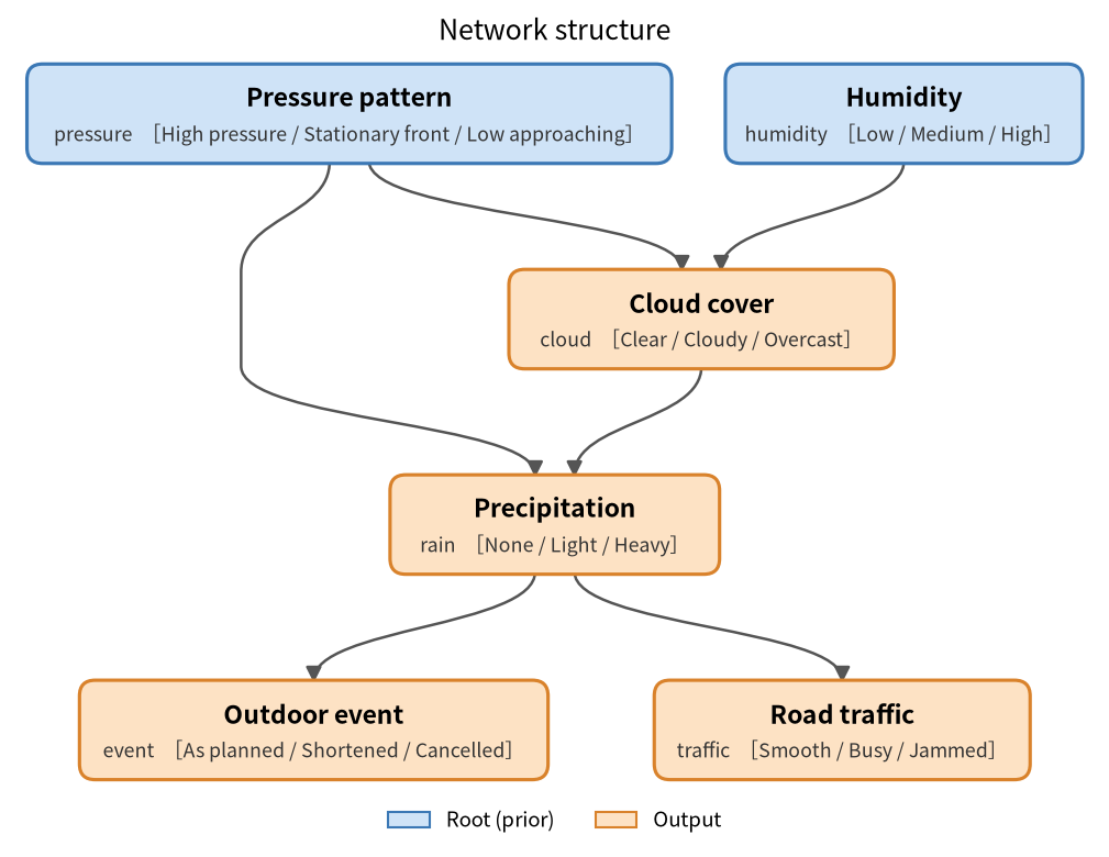
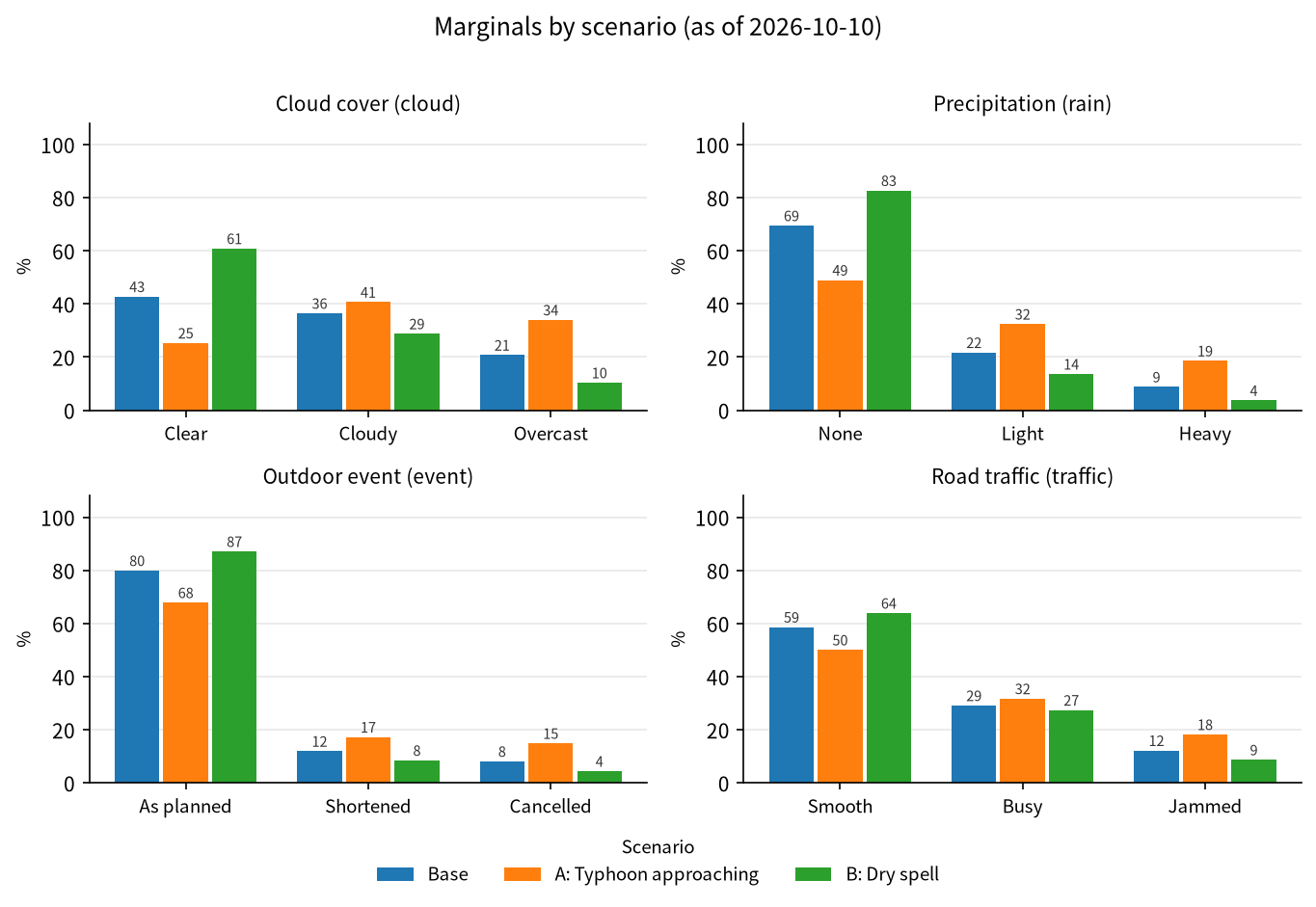
- Scenarios: "A: Typhoon approaching", "B: Dry spell"
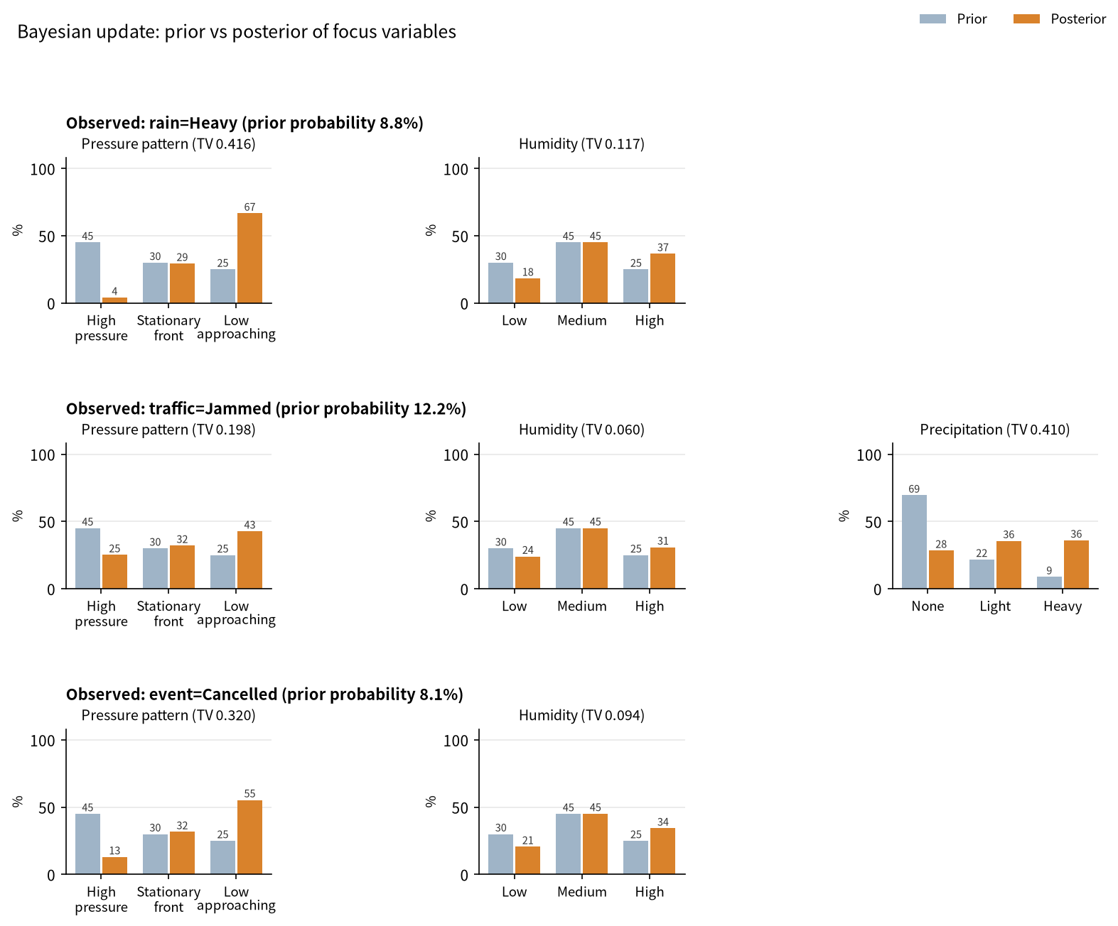
- Observations: infer the pressure pattern and humidity from
rain=Heavy,traffic=Jammed,event=Cancelled
Structure (mermaid; rendered as a diagram on GitHub):
graph TD
  pressure["pressure: Pressure pattern<br/>High pressure/Stationary front/Low approaching"]
  humidity["humidity: Humidity<br/>Low/Medium/High"]
  cloud["cloud: Cloud cover<br/>Clear/Cloudy/Overcast"]
  rain["rain: Precipitation<br/>None/Light/Heavy"]
  event["event: Outdoor event<br/>As planned/Shortened/Cancelled"]
  traffic["traffic: Road traffic<br/>Smooth/Busy/Jammed"]
  pressure --> cloud
  humidity --> cloud
  cloud --> rain
  pressure --> rain
  rain --> event
  rain --> traffic
  classDef root fill:#cfe3f7,stroke:#3b78b5
  class pressure,humidity root
  classDef output fill:#fde2c4,stroke:#d9822b
  class cloud,rain,event,traffic output
Network structure (network.png from --plot):
Marginals by scenario (marginals.png):
Bayesian update, prior vs posterior (updates.png). For example, observing heavy rain raises "Low approaching" for the pressure pattern from 25% to 67%:
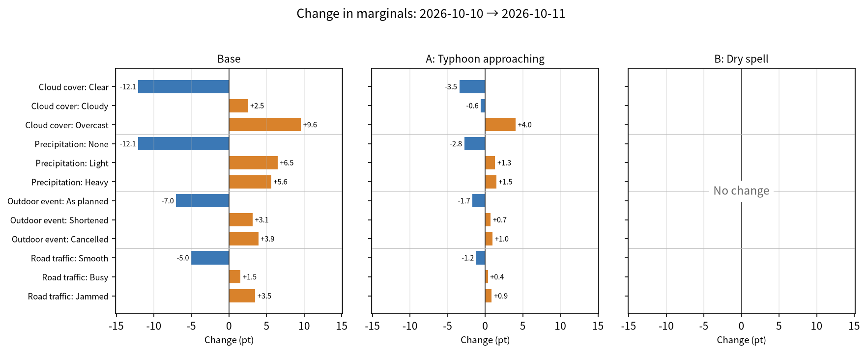
Day-over-day change (diff.png from --diff --plot): the next day, the pressure and humidity priors are revised. Scenarios A and B override the pressure prior (B also humidity), so they change less (B not at all):
Equipment maintenance (examples/maintenance/config.en.json)
- Scenarios: "A: Peak season (high load)", "B: Stronger maintenance"
- Observations: infer load, age and maintenance status from
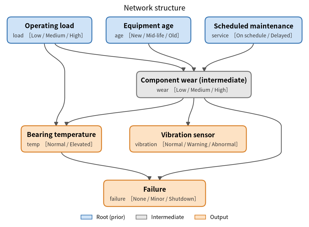
vibration=Abnormal,failure=Shutdown,temp=Elevated wear(component wear) is not inoutputs, so it is an intermediate variable and drawn in grey
graph TD
  load["load: Operating load<br/>Low/Medium/High"]
  age["age: Equipment age<br/>New/Mid-life/Old"]
  service["service: Scheduled maintenance<br/>On schedule/Delayed"]
  wear["wear: Component wear (intermediate)<br/>Low/Medium/High"]
  vibration["vibration: Vibration sensor<br/>Normal/Warning/Abnormal"]
  temp["temp: Bearing temperature<br/>Normal/Elevated"]
  failure["failure: Failure<br/>None/Minor/Shutdown"]
  load --> wear
  age --> wear
  service --> wear
  wear --> vibration
  wear --> temp
  load --> temp
  wear --> failure
  temp --> failure
  classDef root fill:#cfe3f7,stroke:#3b78b5
  class load,age,service root
  classDef middle fill:#e6e6e6,stroke:#777777
  class wear middle
  classDef output fill:#fde2c4,stroke:#d9822b
  class vibration,temp,failure output
Sample output (maintenance, excerpt of --md --lang en):
## failure (Failure)
| Scenario | None | Minor | Shutdown |
|---|---|---|---|
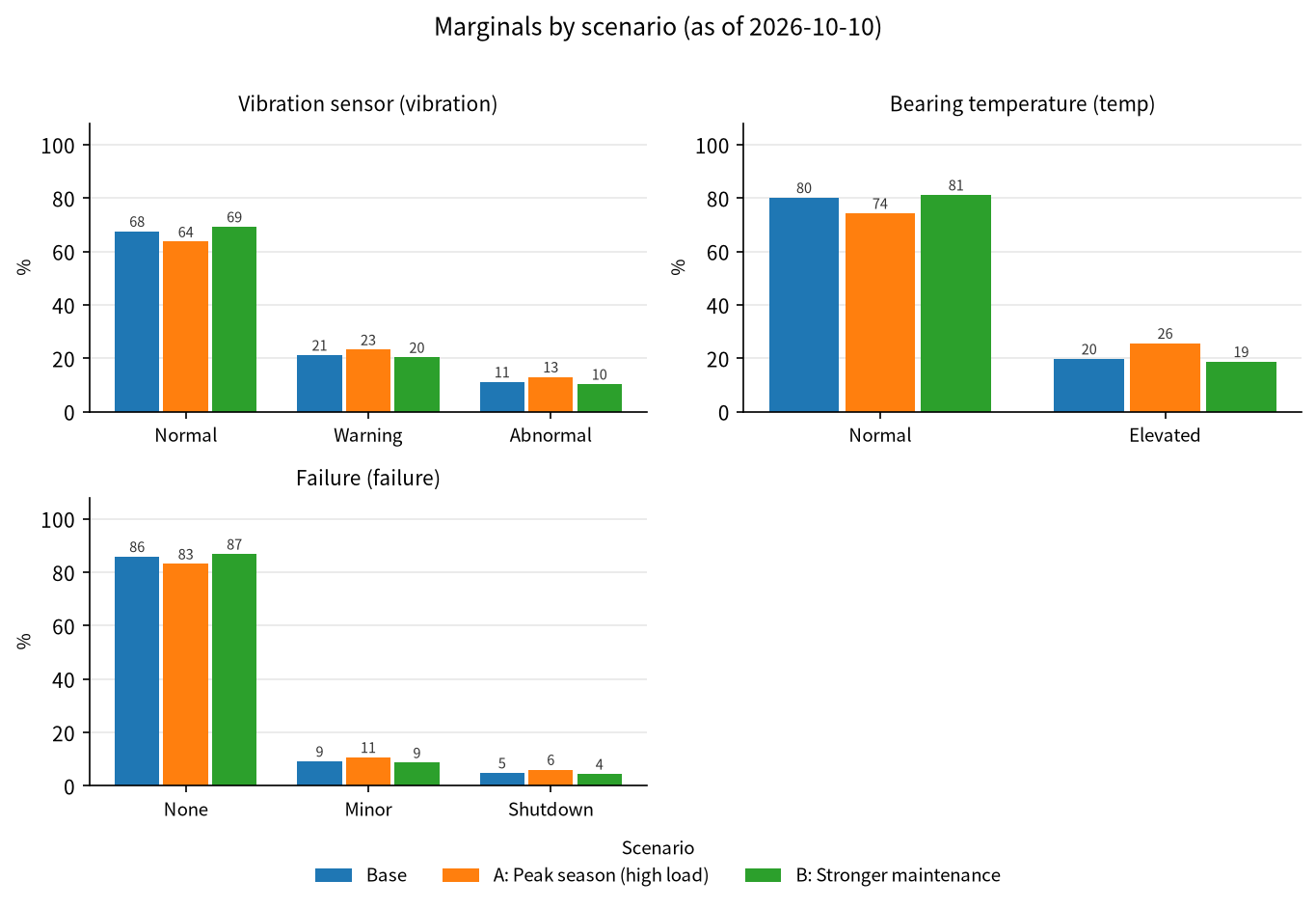
| Base | 85.9% | 9.2% | 4.9% |
| A: Peak season (high load) | 83.2% | 10.7% | 6.1% |
| B: Stronger maintenance | 86.8% | 8.7% | 4.5% |

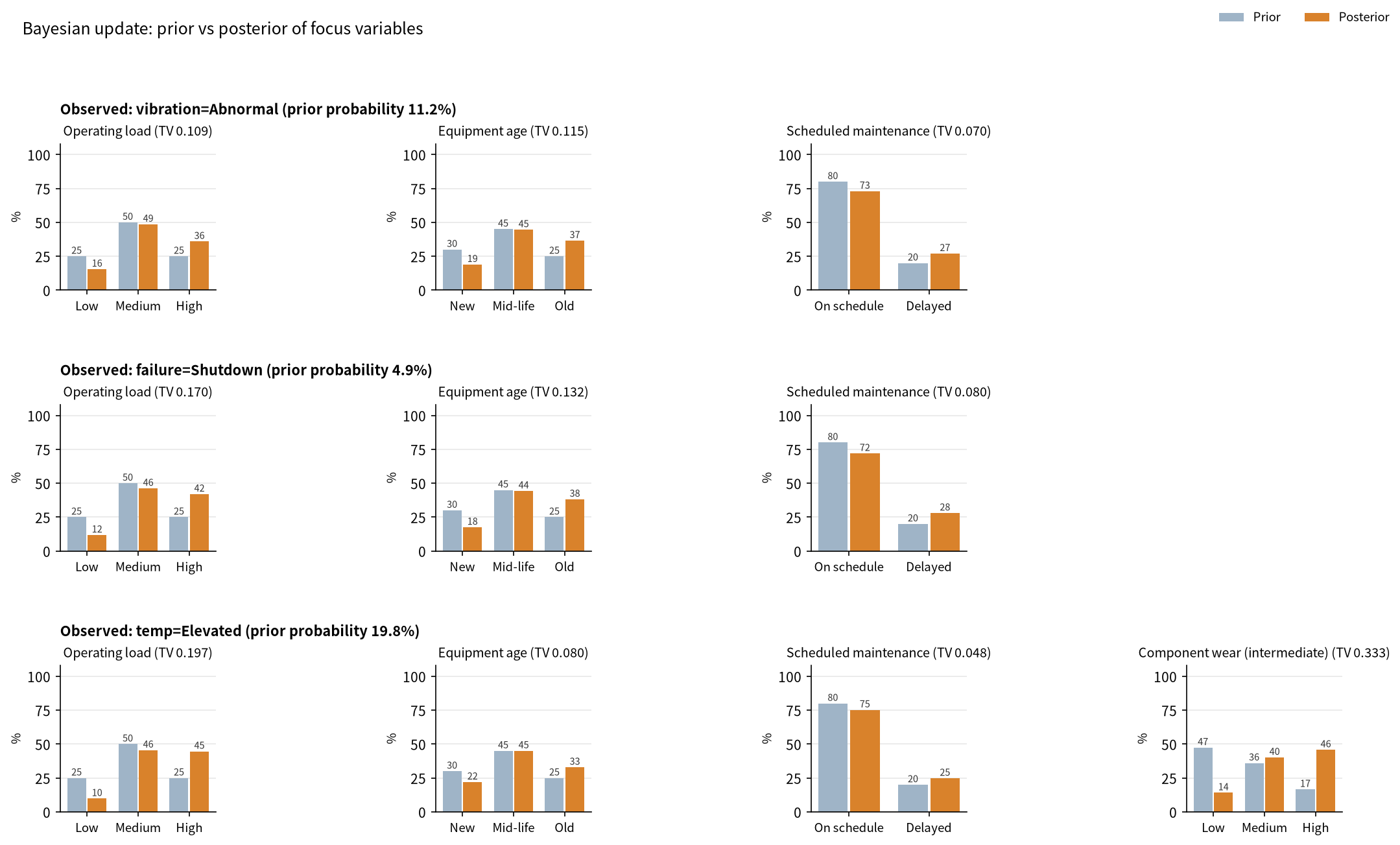
### Observed vibration=Abnormal (prior probability 11.2%)
- wear: Low 8.5% / Medium 32.2% / High 59.3%
- Ranking by movement (TV): age > load > service
Ecology: host–parasite–parasitoid cascade (examples/ecology_host_parasitoid/)
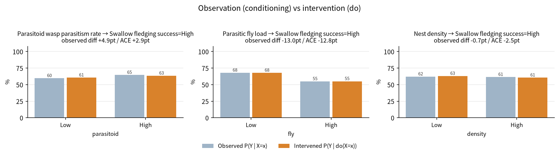
Observation vs intervention with interventions, effects, joint and soft evidence and sensitivity; see its README. All numbers are illustrative placeholders; the topic is inspired by Coroller-Chouraki et al. (bioRxiv, https://doi.org/10.64898/2026.10.06.757064), but the values are not estimates from that paper.
Result keys
By default the keys of results.json are Japanese (unchanged since 0.9). With --json-keys en (or to_english_keys(res) in Python) they are English; names you chose (variables, labels, scenarios, interventions) are never translated, and an observation key X=x を観測 becomes X=x. The default may switch to English in a future major version.
| Japanese | English | Japanese | English |
|---|---|---|---|
基準日 |
as_of |
介入 / 介入内容 |
interventions / do |
シナリオ / 基本 |
scenarios / base |
因果効果 |
effects |
上書き / 周辺 |
overrides / marginals |
P(結果|do(処置)) / P(結果|処置)(観測) |
p_outcome_do / p_outcome_observed |
ベイズ更新(基本) |
updates_base |
ACE / 観測上の差 |
ace / observed_difference |
観測前の確率 / 事後 |
evidence_probability / posterior |
交絡による差(観測上の差−ACE) |
confounding_gap |
証拠 / 尤度 |
evidence / likelihood |
感度分析 / 上位 |
sensitivity / top |
注目変数の事前 / 注目変数の動き |
focus_prior / focus_movement |
幅(pt) |
swing_pt |
動きの大きさ順(TV) |
ranking_by_tv |
検算 |
checks |
The full mapping is fxtensor_bayesnet.keys.KEY_MAP.
Python API
from fxtensor_bayesnet import load_config, run

cfg = load_config("examples/weather/config.en.json")
res = run(cfg)
# result keys are Japanese by default: "シナリオ" = scenarios, "周辺" = marginals, "基本" = base
print(res["シナリオ"]["A: Typhoon approaching"]["周辺"]["rain"])

from fxtensor_bayesnet import to_english_keys, do_config, Engine, Net
en = to_english_keys(res)                      # English keys
print(en["scenarios"]["base"]["marginals"]["rain"])

# joint / soft evidence and do() directly
net = Net(cfg)
priors = {v: cfg["priors"][v]["p"] for v in net.roots}
p_e, post = Engine(net, priors).posterior_raw({"rain": "Heavy", "traffic": {"likelihood": [0.1, 0.3, 0.9]}})
surgered = do_config(cfg, {"cloud": "Overcast"})   # derived config with the kernel of "cloud" replaced

# figures (requires matplotlib)
from fxtensor_bayesnet.plot import plot_all, plot_network
plot_network(cfg, "network.svg", lang="en")
plot_all(res, cfg, "figs", formats=("png",), lang="en")
Layout
src/fxtensor_bayesnet/
  config.py     loading, validation, formatting and hashing of configs
  network.py    building states/kernels with FXTensor; direct einsum computation
  inference.py  marginals per scenario, Bayesian updates (joint / soft evidence), root-cause inference,
                interventions, causal effects, sensitivity, checks
  causal.py     graph surgery (do), effect defaults, one-at-a-time sensitivity
  keys.py       English keys for results JSON
  report.py     Markdown / mermaid output
  history.py    snapshots and diffs
  plot.py       figures (structure, scenarios, updates, changes; matplotlib optional)
  i18n.py       strings for Markdown and figures (Japanese / English)
  cli.py        command line
tests/          pytest
examples/       example configs (Japanese and English; ecology example in English)
docs/images/    README figures (regenerate with docs/make_images.py)
Dependencies
- fxtensor-salmon (MIT License) –
fxtensor-salmon>=1.2.2,<2from PyPI; not vendored. - numpy
- matplotlib (optional,
[plot]) – only for figures
License
MIT License. See LICENSE.
See CHANGELOG.md for the release history.
1 maintainer

Metadata
1 maintainer
Release files for fxtensor-bayesnet 0.10.0
For a detailed explanation of source distributions (sdists) and built distributions (wheels), please see the package formats documentation.
Source distribution (sdist)
| File | Size | Uploaded | |
|---|---|---|---|
| fxtensor_bayesnet-0.10.0.tar.gz | 91.1 kB | Details |
Built distribution (wheel)
| File | Interpreter | ABI | Platform | Reset |
|---|---|---|---|---|
| fxtensor_bayesnet-0.10.0-py3-none-any.whl | Python 3 | none | any | Details |
Total release size: 138.2 kB
Release files / fxtensor_bayesnet-0.10.0.tar.gz
| Download URL | fxtensor_bayesnet-0.10.0.tar.gz |
|---|---|
| Size | 91.1 kB |
| Tags | Source |
|
SHA-256 checksum How to use checksums |
906220c09a6fc7cccfdbc1dd28b68297ff78b0e21bd4ca481d2f30a111df4a8f
|
|
BLAKE2b-256 checksum How to use checksums |
f629ad4a3b6d25a21a48b826ac35706f93f46233d81c47aac85d31c8e33e9e26
|
| Upload date | |
|
Uploaded using Trusted Publishing? What is trusted publishing? |
No |
| Uploaded via |
twine/7.0.0 CPython/3.13.5
|
Release files / fxtensor_bayesnet-0.10.0-py3-none-any.whl
| Download URL | fxtensor_bayesnet-0.10.0-py3-none-any.whl |
|---|---|
| Size | 47.1 kB |
| Tags | Python 3 |
|
SHA-256 checksum How to use checksums |
40ff449609e582e54a588cccdb7fe6f6f94cd64bbc63addcf9312777cc9e4db9
|
|
BLAKE2b-256 checksum How to use checksums |
9be6af0af6209a3ac8d2d67008b78579ec3363f880dcd692bc6b40279a87f8df
|
| Upload date | |
|
Uploaded using Trusted Publishing? What is trusted publishing? |
No |
| Uploaded via |
twine/7.0.0 CPython/3.13.5
|














