Reading a flow rate from Galileo Flow Sensor

Project description
Galileo-Flow SDK is a class based interface to easily communicate with the Galileo Flow Sensor. It contains essential modules to read the flow rate and do other necessary operations.
Setting up the GALILEO Sensor
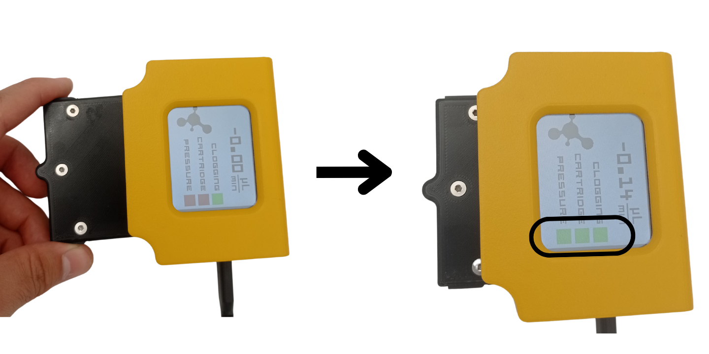
First, insert the cartridge to the base and power on the sensor using type-C USB connector. Make sure that all three flags on the screen are green.
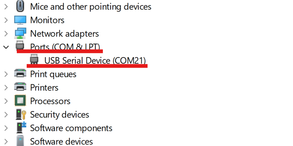
Next, check the COMPORT number of the sensor. In Windows, you can open the Device Manager and find the COMPORT under Ports list:
Example 1. Reading the flow rate
One can use the code snippet below to read the flow rate every second. In your script, instead of 'COM18', do not forget to write the actual comport value.
from GalileoFlowSDK import GalileoFlowSDK
import time

galileo_sensor = GalileoFlowSDK("COM18")
while(1):
    time.sleep(1)
    print('flow is ' , galileo_sensor.read_flow())
Example 2. Reading the liquid type and changing it
The code snippet below allows to check the liquid type in the Galileo Sensor
from GalileoFlowSDK import GalileoFlowSDK

galileo_sensor = GalileoFlowSDK("COM18")
print('liquid is ' , galileo_sensor.read_liquid())
To change the liquid, one can use update_liquid method. The argument ot this method is a number which cooresponds to a liquid type:
- 0: water,
- 1:ip,
- 2:dmem,
- 3:ethanol
For example, in the code below, we set ethanol as a liquid type:
from GalileoFlowSDK import GalileoFlowSDK
import time

galileo_sensor = GalileoFlowSDK("COM18")
galileo_sensor.update_liquid(3)
time.sleep(1)
print('liquid is ' , galileo_sensor.read_liquid())
galileo_sensor.disconnect()
Example 3. Reading the serial number of the Cartridge
Every cartridge has its own unique serial number. This number is useful when utilizing several Galileo Sensors to easily distinguish sensors from each other. In the interface, there is a function to read the serial number:
from GalileoFlowSDK import GalileoFlowSDK
import time
galileo_sensor = GalileoFlowSDK("COM18")
time.sleep(1)
print('Serial number of the cartridge is ' , galileo_sensor.read_serial_number())
galileo_sensor.disconnect()
Example 4. Updating the firmware of the base
The firmware of your base will need to be updated to access to the latest version of Galileo. For that, you will need to upload a binary file called GALILEO_PROJECT.bin (for now, it is sent directly by us when you need an update). Then, you should connect a base with a cartridge, and run the method update_firmware.
Here is an example code to update the firmware and check which firmware version you have. Don't forget to change the path of your binary file to the right location, and to select the right comport.
from GalileoFlowSDK import GalileoFlowSDK
import time

galileo_sensor = GalileoFlowSDK("COM6") #Change to the right comport

while(1):
    command = int(input("command number (1: update firmware, 2: read firmware version) "))
    if command == 1:
        galileo_sensor.update_firmware("C:/Users/Anatole/Downloads/GALILEO_PROJECT.bin")
    elif command == 2:
        print("firmware version: "+galileo_sensor.read_firmware_version())
    else:
        break
Example 5. Setting a feedback loop for flow control using Galileo flow sensor and OB1 pressure controller
This tutorial has been initially written using Windows 10, 64bits, Python 3.8.8 in October, 2021, and modified using Windows 10, 64bits, Python 3.9 in July, 2024. It has been tested using an OB1 mk3+ and a Galileo flow sensor with a range of 0.5 to 20uL/min.
0. Galileo flow sensor addition
Create your main example script and start by importing the GalileoFlowSDK package.
from GalileoFlowSDK import GalileoFlowSDK
import time
1. Elveflow SDK Environment Setup
Make sure you have read all the documentation related to your Elveflow products. Disregarding that information could increase the risk of damage to the equipment, or the risk of personal injuries. In case you don't have a copy, you can download all the documents from Elveflow website.
The content of this chapter of the tutorial is the following:
- Installation
- Instrument configuration
- Instrument calibration
1.1 Installation
The Elveflow Software Development Kit (SDK) latest stable version can be downloaded from the Elveflow website. To alleviate bandwidth and access issues, two links for the same file are provided. You can also find the ESI in the same zip archive file. In case you previously installed the ESI software, a zip folder will also have been added in the same folder of ESI. Unzip it at an easily accessible path as for now, it is necessary to hardcode some paths on the library to customize it for your own system.
Then, go into: '../SDK_V3_08_06/DLL/Python/Python_64' (at the path where you unzipped the SDK), or your equivalent for 32bits, open the file 'Elveflow64.py' with a text editor, edit the fifth line of the code to match the path of your SDK and save your file.
# This python routine load the ElveflowDLL.
# It defines all function prototype for use with python lib

from ctypes import *
ElveflowDLL=CDLL('C:/Users/Anatole/ESI_V3_08_06/SDK_V3_08_06/DLL/DLL64/Elveflow64.dll')# <- change this path
From now on, all the pieces of python scripts written below should be added to the main example script in which you previously imported the GalileoFlowSDK package.
In your main example script, change the paths of the following code cell to match yours and run it. If everything is fine, it should not print any message on the screen.
# tested with Python 3.9 (Pycharm 2023.1.2)
# add python_xx and python_xx/DLL to the project path
# coding: utf8

import sys
from email.header import UTF8

sys.path.append('C:/Users/Anatole/ESI_V3_08_06/SDK_V3_08_06/DLL/DLL64')#add the path of the library here
sys.path.append('C:/Users/Anatole/ESI_V3_08_06/SDK_V3_08_06/DLL/Python/Python_64')#add the path of the LoadElveflow.py

from ctypes import *
from array import array

import matplotlib.pyplot as plt

from Elveflow64 import *
Did you get some outputs? Maybe something is wrong.
In some computers with 64bits, it is necessary to install some additional libraries. To do it, just go again into your SDK folder, find the path '../SDK_V3_08_06/Extra Install For x64 Libraries' and run the setup application that you will find inside. Then, try to launch again the previous code cell.
1.2 Instrument configuration
Once the SDK has been correctly installed, it is also necessary to configure it to work with the desired system. Depending on the version of your OB1, you will need to know either the OB1 name, or the comport your OB1 is connected to.
1.2.1 Finding OB1 name
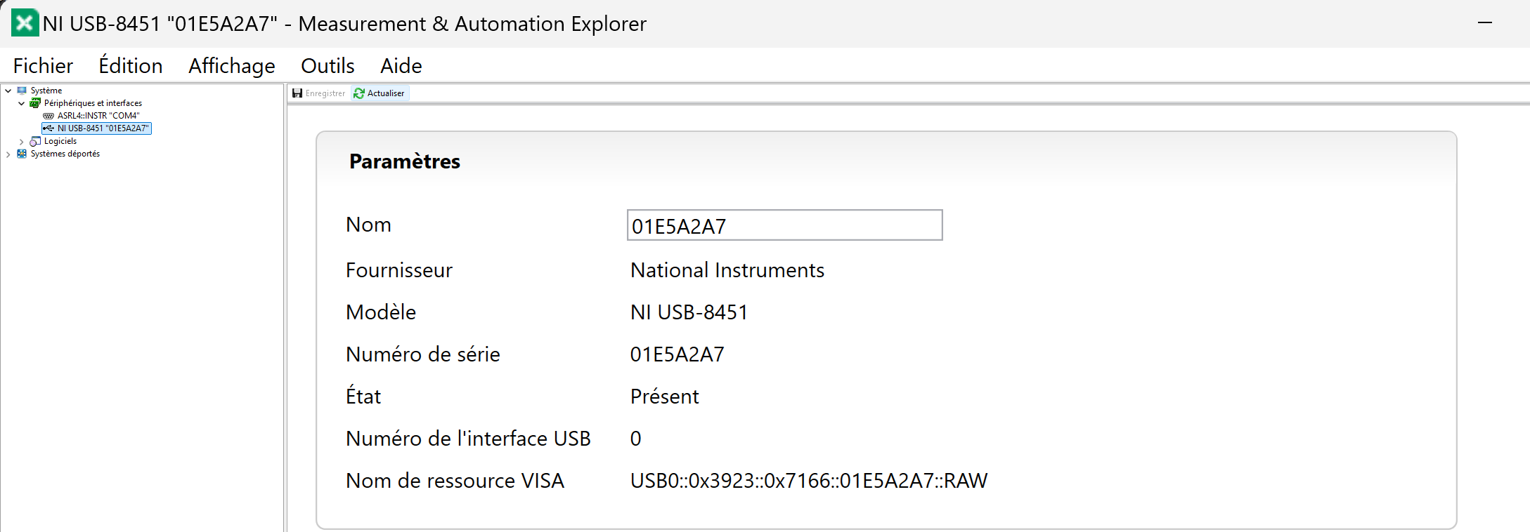
If you previously installed the ESI, an application called NI MAX should have been installed as well. It is needed to check the exact name of the device.
How? First, connect your device to the power supply, connect its USB cable to the computer you are using and turn it on. After that, go to Windows search bar and type 'NI MAX' without the quotes.
Then, just unzip the left tabs: 'My System > Devices and Interfaces'.
If you don't have more National Instrument's devices connected to your computer, the only result should be the OB1 Pressure Controller (or the one that you try to configure). Click on it and write down its Serial Number. You will need it for your custom software to interact with the device. In this example (in french here), the device Serial Number is 01E5A2A7.
1.2.2 Finding OB1 comport
The comport number can be found in the Device Manager.
1.2.3 Pressure regulators encoding
The next step is to know the arrangement of pressure regulators that your system has. In order to identify them, you can check it on the OB1 User guide, at the installation chapter.
Each regulator has a different encoding value (between 0 and 5). The correspondance is the following:
- Non-installed : 0
- (0, 200) mbar : 1
- (0, 2000) mbar : 2
- (0, 8000) mbar : 3
- (-1000, 1000) mbar : 4
- (-1000, 6000) mbar : 5
At max, the OB1 controller will have four pressure outputs, thus, in the OB1_Initialization() call of the following code cell, after the serial number, you must specify the regulator type of every channel, setting a zero if a channel is not physically installed. In the following code, four pressure outputs are installed with regulators of type 1 and 2.
# Initialization of OB1

Instr_ID = c_int32()
print("Instrument name and regulator types are hardcoded in the Python script")

# See User Guide to determine regulator types and NIMAX to determine the instrument name
error = OB1_Initialization('01E5A2A7'.encode('ascii'),1,2,2,2,byref(Instr_ID))

# All functions will return error codes to help you to debug your code, for further information refer to User Guide
print('error:%d' % error)
print("OB1 ID: %d" % Instr_ID.value)
If everything went fine, you should have received a simple message as follows:
Instrument name and regulator types are hardcoded in the Python script
error:0
OB1 ID: 0
If it is not the case, one or several of the following issues can be happening:
- The OB1 is not connected to the power supply or to the computer through the USB wire.
- The OB1 is not on. The screen should emit blue light.
- The Serial Number or Com Port of the device was not correctly written.
- There are several instances trying to reach the OB1. Close any ESI window running and be sure of using only one python script (of OB1 interfacing code) at a time.
- If you installed extra libraries, try restarting your computer.
- The USB wire may need to be unplugged and plugged or changed to another USB port.
1.3 Instrument calibration
Here you can choose, essentially, one of the three available options: default, load and new. The calibration consists of an array which stores the actual values associated to your instrument.
If you previously proceeded with a calibration process, you can load it from the Calib_path that you must previously specify. Otherwise, if you want to run a calibration process, ensure that ALL channels are properly closed with adequate caps. You can find more detailed instructions about the calibration procedure at the OB1 User Guide.
Calib = (c_double*1000)() # Always define array this way, calibration should have 1000 elements

while True:
    answer = input('select calibration type (default, load, new ) : ')
    Calib_path = 'C:\\Users\\Public\\Desktop\\Calibration\\Calib.txt'
    if answer == 'default':
        error = Elveflow_Calibration_Default (byref(Calib),1000)
        break

    if answer == 'load':
        error = Elveflow_Calibration_Load (Calib_path.encode('ascii'), byref(Calib), 1000)
        break

    if answer == 'new':
        OB1_Calib (Instr_ID.value, Calib, 1000)
        error = Elveflow_Calibration_Save(Calib_path.encode('ascii'), byref(Calib), 1000)
        print('Calib saved in %s' % Calib_path.encode('ascii'))
        break
The expected output would be something like:
select calibration type (default, load, new ) : default
Here finishes the first part of this tutorial. The next part continues the script to implement the automatic PI control.
2. Automatic PI Control
In this part of the tutorial, the basic process for setting up an automatic control is shown. It is assumed that you have correctly set up the SDK environments as it was shown in chapters 0 and 1 of the tutorial. If you didn't see it before, please, go for it first.
The content of this chapter of the tutorial is the following:
- PI basics
- PI software
- Parameters tuning
2.1 PI basics
The PI Controller or Proportional-Integrative Controller is a basic linear controller, yet powerful for lot of situations, which makes the output of the controlled system to follow a desired curve of values, called reference, and ensures that the system properly works and that it is stable for the operating expected situation.
To achieve this control of the system's output, it takes the current system's output value, calculates the difference to the reference (the desired output), which is called error, and makes some operations with it.
The operations for a basic PI Control are two: the proportional term calculus and the integrative term calculus.
The proportional term corresponds to the current error multiplied by a proportional gain $K_p$. The larger this gain is, the more aggressive the control will react. For an instant k:
$$P_{term} = K_p(y_k-y_{ref})$$
The integrative term corresponds to the accumulated error multiplied by an integrative gain $K_i$. The larger this gain is, the faster the control will react to the changes between the real output and the desired one. For an instant k:
$$I_{term} = K_i \sum_{j=0}^{k} (y_j-y_{ref})$$
Note. Usually, the integrative gain is expressed as integrative time which is related to the integrative gain through the sampling period of the controlling system, but it is shown here this way as may be considered more understandable with gains.
2.2 PI software
In the following code, there are two functions which run the control over the system.
If your microfluidic circuit is not very hydraulically resistive, you may need to add some flow resistance to it in order to make use of the whole ranges of your flow sensor and pressure regulators.
flow_list = []
error_list = []
control_list = []
p_error = 0
i_error = 0
meas_flow = c_double()
def pid_run():
global p_error
global i_error
start_t = time.time() # <- This must be close to the routine
last_t = start_t
# Main routine
while True:
# Get the current output
flow_list.append(galileo_flow.read_flow())
# Calculate the mathematical error
p_error = ref_flow - galileo_flow.read_flow()
i_error += p_error
i_error = min(i_error, i_max)
# PI Controller equations
P_val = K_p * p_error
I_val = K_i * i_error
p_control = P_val + I_val
p_control = max(p_min, min(p_max, p_control)) # Safety saturation
error_list.append(p_error)
control_list.append(p_control)
p_control = c_double(float(p_control)) # Convert to c_double
error = OB1_Set_Press(Instr_ID.value, pchannel, p_control, byref(Calib), 1000) # Return error message.value, p_channel, p_control, byref(Calib), 1000) # Return error message
# Check if the elapsed time match the time limit
if (time.time() - start_t) > experiment_t:
break
# Wait until desired period time
sleep_t = period - (time.time() - last_t)
if sleep_t > 0:
time.sleep(sleep_t)
last_t = time.time() # And update the last time
# Turn off the pressure
p_control = 0.0
error = OB1_Set_Press(Instr_ID.value, pchannel, p_control, byref(Calib), 1000) # Return error message.value, p_channel, p_control, byref(Calib), 1000) # Return error message
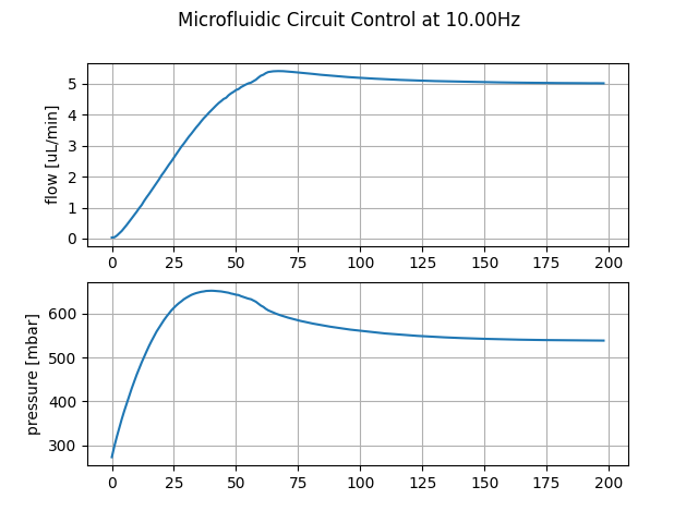
def plot():
# Plot the signals
plt.rcParams['axes.grid'] = True
fig = plt.figure()
fig.suptitle("Microfluidic Circuit Control at {0:.2f}Hz".format(1 / period))
plt.subplot(2, 1, 1)
plt.plot(flow_list)
plt.ylabel('flow [uL/min]')
plt.subplot(2, 1, 2)
plt.plot(control_list)
plt.ylabel('pressure [mbar]')
plt.show()
def run():
pid_run()
plot()
2.3 Parameters tuning
Each microfluidic system needs a different PI Controller tuning, thus, the results you will have may be different to the ones obtained with our testing setup.
Change the following values to tune the controller for your system. You can also change the reference value and the experiment execution time by some values more useful for your application. If the system follows your reference too slowly, you may increase the proportional and/or the integrative gain. If it is too aggressive, the contrary. Feel free to play with them by changing the values in small steps.
Important: check that the control maximum and minimum values are good for your system.
galileo_flow = GalileoFlowSDK("COM4") #Change this to the correct com port

# Controller parameters:

period = 0.1 # 10Hz

K_p = 50 # <- Change this value to tune the controller
K_i = 5 # <- Change this value too to tune the controller
ref_flow = 5 # uL/min

p_min = 0 # <- This is only negative if you have some vacuum source
p_max = 2000 # <- This depends on the regulator of each channel
i_max = p_max / (K_i)

# OB1 arrangement
pchannel = 2 # <- Change this to your real configuration

experiment_t = 10.0 # Seconds
flow_list = []
error_list = []
control_list = []

run()
Conclusion
In this tutorial we have seen how a simple PI Control works, how can it be implemented with the Galileo flow sensor and the OB1 instrument and how to tune its parameters.
Hope you found this tutorial useful !


Download files
Download the file for your platform. If you're not sure which to choose, learn more about installing packages.
Source Distributions
Built Distribution
Filter files by name, interpreter, ABI, and platform.
If you're not sure about the file name format, learn more about wheel file names.
Copy a direct link to the current filters
File details
Details for the file GalileoFlowSDK-0.1.6-py3-none-any.whl.
File metadata
- Download URL: GalileoFlowSDK-0.1.6-py3-none-any.whl
- Upload date:
- Size: 13.0 kB
- Tags: Python 3
- Uploaded using Trusted Publishing? No
- Uploaded via: twine/5.1.1 CPython/3.8.2
File hashes
| Algorithm | Hash digest | |
|---|---|---|
| SHA256 |
2b0ac281db4af8eb72b9416d698a67fee740f6b4285837792ae1320c764e99c4
|
|
| MD5 |
a050118f7c029f6c3153d0fbb47a9270
|
|
| BLAKE2b-256 |
cfbbc98319f1583ac0c4ef40e0bc1b1efd107ce9bdb545432b2472ddda0bb8e0
|


