Pure-Python spatial analysis toolkit with GeoJSON-native geometries and GeoPandas-style frame workflows.

Project description
GeoPrompt
A pure-Python spatial analysis toolkit providing 530 geospatial tools for point, line, and polygon workflows. GeoPrompt delivers GeoPandas-style frame access, GeoJSON-compatible I/O, CRS-aware reprojection, spatial joins, geographic distance methods, and a comprehensive suite of spatial statistics, interpolation, clustering, terrain analysis, network routing, AI-powered analysis, pseudo-quantum computing, optimal transport, topological analysis, graph diffusion, conformal prediction, and interchange formats.
Key Features
- 530 spatial analysis tools covering interpolation, classification, clustering, regression, terrain analysis, network analysis, point patterns, geometry utilities, I/O formats, raster operations, AI/ML methods, pseudo-quantum algorithms, optimal transport, topological inference, graph dynamics, and more
- Pure-Python package code — published as a universal wheel; optional extras integrate with heavier geospatial and statistical stacks when needed
- GeoJSON-native — all geometries use standard GeoJSON format internally
- CRS-aware — coordinate reference system assignment and reprojection via
to_crs() - Scientifically grounded — algorithms validated against Shapely, SciPy, NumPy, PySAL, PyKrige, GeoPandas, scikit-learn, and statsmodels
Installation
pip install geoprompt
For optional support libraries and reference-grade comparisons:
pip install geoprompt[compare,overlay,projection]
pip install geoprompt[io,raster]
Install Notes
pip install geopromptinstalls the base package and core plotting dependency.pip install geoprompt[compare]adds reference-comparison libraries such as PySAL, GeoPandas, PyKrige, Shapely, and statsmodels.pip install geoprompt[overlay,projection]adds geometry overlay and CRS transformation support.pip install geoprompt[io,raster]adds Fiona, OpenPyXL, PyShp, and Rasterio for broader file-format and raster workflows.- Optional extras may pull in compiled third-party wheels depending on platform.
Quick Start
import geoprompt as gp

# Load spatial data
frame = gp.read_features("sites.geojson", crs="EPSG:4326")

# Run spatial analysis
hotspots = frame.hotspot_getis_ord(
    value_column="population",
    mode="distance_band",
    max_distance=5000,
    fdr_correction=True,   # Benjamini-Hochberg multiple testing correction
)

# Interpolate a surface
surface = frame.kriging_surface(
    value_column="elevation",
    grid_resolution=50,
    auto_fit_variogram=True,  # automatic variogram model fitting
)

# Cluster analysis
clusters = frame.optics_clustering(min_samples=5)
Accuracy & Validation
GeoPrompt maintains an evidence-based accuracy posture. Each tool is classified by maturity level:
| Level | Meaning |
|---|---|
| Deterministic | Direct transformation with provably correct output |
| Validated | Cross-validated against reference implementations (Shapely, SciPy, PySAL) |
| Approximation | Operationally useful; lightweight implementation of a fuller algorithm |
| Heuristic | Optimization shortcut — useful but not guaranteed globally optimal |
Tool Reference
This section is a curated reference to major tool families. The full machine-readable inventory is available in docs/tool-inventory.json.
Interpolation & Surface Analysis (Tools 12–13, 53, 80, 191–193, 199)
| Tool | Method | Key Parameters |
|---|---|---|
idw_interpolation |
Inverse Distance Weighting | power, search_radius, k_neighbors |
kriging_surface |
Ordinary Kriging with auto-fit variogram | auto_fit_variogram, variogram_model |
natural_neighbor_interpolation |
Sibson-style area-weighted interpolation | grid_resolution |
spline_interpolation |
Thin-plate spline | grid_resolution, smoothing |
kriging_cross_validation |
Leave-one-out CV for kriging quality | Returns RMSE, MAE |
adaptive_idw |
IDW with LOO cross-validated local power | k_neighbors, powers |
conformal_kriging |
Spatially calibrated conformal kriging intervals | calibration_fraction, alpha, local_k |
raster_algebra |
Safe math expression on grid values | expression (uses x) |
space_time_kriging |
Product-sum variogram space-time kriging | value_column, time_column |
Classification & Clustering (Tools 3, 41–43, 77–79, 90, 98, 187–188, 529)
| Tool | Method | Key Parameters |
|---|---|---|
centroid_cluster |
K-means with silhouette scoring | k, max_iterations |
dbscan_cluster |
Density-based clustering | epsilon, min_samples |
hierarchical_cluster |
Agglomerative clustering | k, linkage |
optics_clustering |
Density-based with variable epsilon | min_samples, xi |
jenks_natural_breaks |
Fisher-Jenks classification | k (number of classes) |
equal_interval_classify |
Equal-width binning | k |
quantile_classify |
Equal-count binning | k |
location_allocation |
P-median facility optimization | p, demand_column |
dbscan |
DBSCAN with true distance matrix | eps, min_samples |
hdbscan |
Hierarchical DBSCAN via mutual reachability MST | min_cluster_size |
network_constrained_clustering |
Connected k-medoids over a k-NN graph | n_clusters, k, max_iterations |
Spatial Statistics (Tools 10–11, 16–17, 52, 72–76, 86–87, 89, 91, 189–190, 521, 523, 527–528)
| Tool | Method | Key Parameters |
|---|---|---|
spatial_autocorrelation |
Global Moran's I | mode, permutations |
spatial_lag |
Spatial lag computation | mode, k, max_distance |
hotspot_getis_ord |
Local Gi* with optional FDR correction | fdr_correction, alpha |
local_outlier_factor_spatial |
LOF anomaly detection | k, outlier_threshold |
ripleys_k |
Ripley's K with edge correction | edge_correction, steps |
bivariate_morans_i |
Bivariate spatial correlation | x_column, y_column |
local_gearys_c |
Local dissimilarity measure | mode, k |
spatial_scan_statistic |
Kulldorff cluster detection | n_simulations, max_radius_fraction |
geographic_detector |
Wang-Xu factor detector (q-statistic) | factor_column |
nearest_neighbor_index |
Clark-Evans NNI | Returns ratio, z-score |
spatial_outlier_zscore |
Local spatial z-score | k, threshold |
transport_aware_hotspot |
Accessibility-weighted adaptive hotspot detection | value_column, supply_column, beta |
global_gearys_c |
Global Geary's C | mode, k |
morans_i_local |
Local Moran's I (LISA) | mode, permutations |
mark_correlation_function |
Mark dependence vs distance | mark_column, steps |
point_pattern_intensity |
First-order λ(s) surface | kernel_bandwidth |
multivariate_morans_i |
Cross-variable Moran's I matrix | columns, k |
local_geary_decomposition |
Multivariate local Geary statistic | columns, k |
topologically_regularized_spatial_scan |
Contiguity-penalized Kulldorff scan | topo_penalty, adjacency_k |
wavelet_spatial_autocorrelation |
Multi-scale wavelet decomposition autocorrelation | n_scales, base_bandwidth |
multiscale_getis_ord |
Gi* across multiple distance bands | scales, n_scales |
Regression (Tools 21–22, 88, 99, 197–198, 522, 526)
| Tool | Method | Key Parameters |
|---|---|---|
spatial_regression |
OLS with spatial diagnostics | independent_columns |
geographically_weighted_summary |
GWR with CV bandwidth & local R² | auto_bandwidth, bandwidth |
loess_regression |
LOESS (local polynomial smoothing) | fraction, degree |
spatial_durbin_model |
SDM with spatial lags of X and Y | mode, k |
negative_binomial_gwr |
GW negative binomial regression (IRLS) | independent_columns, bandwidth |
counterfactual_gwr |
GWR with counterfactual scenario analysis | scenario, auto_bandwidth |
geographically_weighted_pca |
Local PCA with spatial weights | columns, n_components |
spatial_durbin_error_model |
SDEM with spatial error & lag-X spillovers | lambda_init, max_iter |
Density & Surface (Tools 18–19, 97, 525)
| Tool | Method | Key Parameters |
|---|---|---|
kernel_density |
KDE with Silverman bandwidth & kernel selection | kernel (epanechnikov, gaussian, quartic) |
standard_deviational_ellipse |
Weighted covariance ellipse | weight_column |
point_pattern_intensity |
Kernel-smoothed intensity surface | grid_resolution |
anisotropic_kernel_density |
Oriented Gaussian KDE with major/minor axes | bandwidth, angle_column, ratio |
Regionalization (Tools 129, 160–161, 262, 271, 287, 297–298, 524)
| Tool | Method | Key Parameters |
|---|---|---|
max_p_regions |
Regionalization with endogenous region count | floor_variable, floor_value |
skater_regionalization |
MST-based regionalization | attribute_columns, n_regions |
azp_regionalization |
Automatic zoning procedure | attribute_columns, n_regions |
soft_regionalization |
Fuzzy region membership assignment | attribute_columns, n_regions |
regionalization_stability |
Region stability under perturbations | attribute_columns, n_regions, n_runs |
regionalization_diagnostics |
Region compactness and balance review | label_column |
regionalization_consensus |
Consensus labels from multiple partitions | label_columns |
region_adjacency_summary |
Adjacency and border statistics by region | label_column |
graph_coupled_space_time_regionalization |
Contiguous regions balancing spatial and temporal dissimilarity | value_columns, time_column, n_regions |
Terrain & Hydrology (Tools 7–8, 92–95)
| Tool | Method | Key Parameters |
|---|---|---|
slope_aspect |
Slope and aspect from surface model | grid_resolution |
hillshade |
Terrain illumination model | azimuth, altitude |
terrain_ruggedness_index |
RMS elevation change to neighbors | elevation_column |
topographic_position_index |
Relative elevation with landform class | k |
flow_direction |
D8 steepest-descent routing | elevation_column |
flow_accumulation |
Upslope contributing area | elevation_column |
stream_power_index |
SPI erosive power proxy | elevation_column, k |
Network Analysis (Tools 31–40, 171, 195–196)
| Tool | Method |
|---|---|
network_build |
Corridor-to-graph edge/node construction |
shortest_path |
Dijkstra routing with diagnostics |
service_area |
Reachable-edge extraction with partial coverage |
location_allocate |
Network-cost demand assignment with capacity |
corridor_reach |
Route-proximity screening with scoring |
origin_destination_matrix |
Pairwise Dijkstra cost matrix |
k_shortest_paths |
Best-first simple-path enumeration |
network_trace |
Forward/reverse breadth-first traversal |
route_sequence_optimize |
Greedy nearest-next + 2-opt refinement |
snap_to_network_nodes |
Nearest-node assignment |
service_area_polygons |
Dijkstra reachability → convex hull polygons |
isochrones |
Travel-time contour rings from network origin |
network_betweenness |
Brandes betweenness centrality on k-NN graph |
Anomaly Detection (Tools 406, 455, 473, 475, 478, 530)
| Tool | Method | Key Parameters |
|---|---|---|
spatial_anomaly_detector |
Isolation-forest-style anomaly detection | columns, contamination |
spatial_outlier_ensemble |
Ensemble outlier scoring from multiple local diagnostics | value_column, k |
spatial_bootstrap_confidence |
Bootstrap local uncertainty and tail-risk flags | value_column, n_bootstrap |
spatial_permutation_test |
Monte Carlo anomaly/significance screening | value_column, n_permutations |
spatial_silhouette_score |
Cluster-separation anomaly diagnostic | label_column, distance_method |
spatial_envelope_anomaly |
Local multivariate envelope exceedance scoring | value_columns, k, contamination |
Geometry Operations (Tools 23–30, 44–51, 194)
| Tool | Method |
|---|---|
buffer |
Point/Line/Polygon buffering |
dissolve |
Attribute-based geometry union |
clip |
Geometry intersection clipping |
overlay_intersections |
Pairwise intersection extraction |
overlay_union |
Face partitioning with lineage |
erase |
Geometry difference |
simplify |
Douglas-Peucker simplification |
densify |
Segment subdivision |
smooth_geometry |
Chaikin smoothing |
multipart_to_singlepart |
Explode multipart geometries |
singlepart_to_multipart |
Group and union |
eliminate_slivers |
Area/vertex threshold filtering |
convex_hulls / envelopes |
Geometry bounds |
polygon_triangulation |
Ear-clipping polygon triangulation |
Raster-like Operations (Tools 1–9)
| Tool | Method |
|---|---|
raster_sample |
Nearest/IDW lookup at query locations |
zonal_stats |
Point-in-polygon aggregation |
reclassify |
Attribute mapping or break classification |
resample |
Spatial thinning or random subset |
raster_clip |
Bounds intersection filter |
mosaic |
Row merge with conflict resolution |
to_points / to_polygons |
Geometry conversion |
contours |
Marching-squares isoline extraction |
Trajectory & Change Detection (Tools 56–60)
| Tool | Method |
|---|---|
trajectory_match |
GPS-to-network matching |
trajectory_staypoint_detection |
Radius-duration grouping |
trajectory_simplify |
Douglas-Peucker on trajectories |
spatiotemporal_cube |
Space-time binned aggregation |
change_detection |
Feature-level temporal differencing |
Encoding & Utilities (Tools 61–71, 81–85)
| Tool | Method |
|---|---|
geohash_encode |
Geohash string generation |
thiessen_polygons |
Voronoi partitioning (Shapely-accelerated) |
spatial_weights_matrix |
Dense pairwise neighbor weights |
zone_fit_score |
Multi-factor zone matching with scoring |
random_points |
Random point generation within bounds |
I/O & Interchange (Tools 145–148, 200–201)
| Tool | Method |
|---|---|
read_shapefile / to_shapefile |
ESRI Shapefile import/export |
read_geopackage |
OGC GeoPackage import |
read_kml |
KML import |
to_topojson |
TopoJSON export |
read_geoparquet / to_geoparquet |
GeoParquet import/export via GeoPandas |
read_flatgeobuf / to_flatgeobuf |
FlatGeobuf import/export via GeoPandas |
Usage Examples
Loading Data
import geoprompt as gp

# From GeoJSON files
frame = gp.read_features("sites.geojson", crs="EPSG:4326")

# From in-memory records
frame = gp.GeoPromptFrame.from_records([
    {"site_id": "HQ", "geometry": {"type": "Point", "coordinates": [-111.95, 40.71]}, "population": 5000},
    {"site_id": "Branch", "geometry": {"type": "Point", "coordinates": [-111.90, 40.68]}, "population": 2000},
], crs="EPSG:4326")

# Random point generation for testing
random_pts = gp.GeoPromptFrame.random_points(count=1000, min_x=-112, max_x=-111, min_y=40, max_y=41, seed=42)
Spatial Statistics
# Hotspot analysis with FDR correction
hotspots = frame.hotspot_getis_ord(
    value_column="population",
    mode="distance_band",
    max_distance=5000,
    fdr_correction=True,
    alpha=0.05,
)

# Spatial autocorrelation
autocorr = frame.spatial_autocorrelation("population", mode="k_nearest", k=4, permutations=99)
report = autocorr.report_autocorrelation_patterns("population")

# Bivariate Moran's I
bivar = frame.bivariate_morans_i("income", "education", mode="k_nearest", k=4)

# Spatial scan statistic (Kulldorff)
scan = frame.spatial_scan_statistic("cases", "population", n_simulations=99)
Interpolation
# Kriging with automatic variogram fitting
surface = frame.kriging_surface(
    value_column="elevation",
    grid_resolution=50,
    auto_fit_variogram=True,
)

# Cross-validate kriging quality
cv = frame.kriging_cross_validation(value_column="elevation")
print(f"RMSE: {cv['rmse']:.3f}, MAE: {cv['mae']:.3f}")

# IDW with search radius
idw = frame.idw_interpolation("temperature", grid_resolution=30, search_radius=10.0, k_neighbors=12)

# Kernel density with Silverman bandwidth
kde = frame.kernel_density(weight_column="incidents", kernel="gaussian", grid_resolution=40)
Regression
# Geographically weighted regression with auto-bandwidth
gwr = frame.geographically_weighted_summary(
    dependent_column="price",
    independent_columns=["sqft", "bedrooms"],
    auto_bandwidth=True,
)

# Spatial Durbin Model
sdm = frame.spatial_durbin_model("price", ["sqft", "bedrooms"], mode="k_nearest", k=4)

# LOESS smoothing
loess = frame.loess_regression("temperature", "elevation", fraction=0.3)
Clustering & Classification
# OPTICS density clustering
clusters = frame.optics_clustering(min_samples=5, xi=0.05)

# P-median facility location
facilities = frame.location_allocation(demand_column="population", p=5, seed=42)

# Jenks natural breaks
classified = frame.jenks_natural_breaks("income", k=5)
Terrain & Hydrology
# Terrain analysis
tri = frame.terrain_ruggedness_index("elevation")
tpi = frame.topographic_position_index("elevation", k=8)

# Hydrological routing
flow_dir = frame.flow_direction("elevation")
flow_acc = frame.flow_accumulation("elevation")
Network Analysis
# Build a routable network from line features
network = corridors.network_build()

# Shortest path routing
route = network.shortest_path(origin="node-A", destination="node-B")

# Service area analysis
service = network.service_area(origins=["depot-1"], max_cost=5000)

# Origin-destination cost matrix
od_matrix = network.origin_destination_matrix(origins=["A", "B"], destinations=["X", "Y"])
Geometry Operations
# Spatial join
joined = regions.spatial_join(assets, predicate="contains")

# Buffer and dissolve
buffered = frame.buffer(distance=100)
dissolved = frame.dissolve(by="region", aggregations={"population": "sum"})

# Overlay operations
clipped = assets.clip(regions)
intersections = regions.overlay_intersections(assets)
Project Structure
geoprompt/
├── src/geoprompt/
│   ├── __init__.py          # Public API exports
│   ├── frame.py             # GeoPromptFrame class — all 530 spatial tools
│   ├── geometry.py          # Geometry primitives and helpers
│   ├── equations.py         # Shared mathematical functions
│   ├── overlay.py           # Polygon overlay operations
│   ├── compare.py           # Shapely/GeoPandas comparison utilities
│   ├── spatial_index.py     # R-tree spatial index
│   ├── demo.py              # Demo runner
│   └── io.py                # GeoJSON, CSV, and records I/O
├── assets/                  # Demo images
├── pyproject.toml
├── CHANGELOG.md
├── CONTRIBUTING.md
└── README.md
Running Tests
pytest --tb=short -q
CI validation is defined in .github/workflows/geoprompt-ci.yml.
License
MIT
Custom Equations
- Prompt decay:
1 / (1 + distance / scale) ^ power - Prompt influence:
weight * prompt_decay(distance, scale, power) - Prompt interaction:
origin_weight * destination_weight * prompt_decay(distance, scale, power) - Corridor strength:
weight * log(1 + corridor_length) * prompt_decay(distance, scale, power) - Area similarity:
min(area_a, area_b) / max(area_a, area_b) * prompt_decay(distance, scale, power)
These are intentionally simple first equations. The package now supports two distance modes:
euclideanfor planar coordinate space and direct comparison with Shapely and GeoPandas raw-coordinate resultshaversinefor geographic point-to-point distances in kilometers when your coordinates are longitude/latitude
The package now supports CRS tagging and reprojection, but it is still designed so richer CRS handling, overlays, and additional operators can be layered in later.
Package Interface
The main package entry points are:
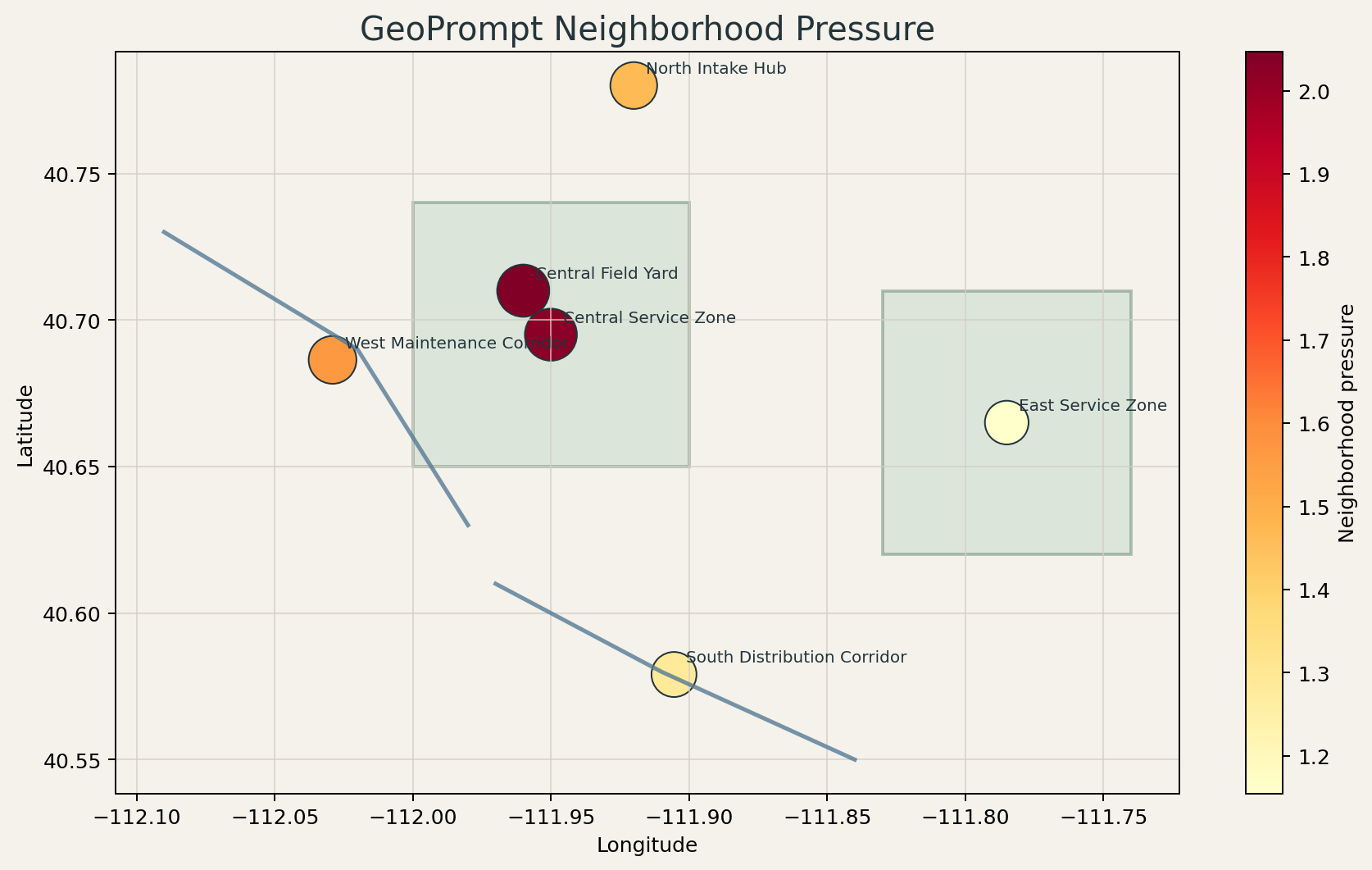
geoprompt.read_points(...)geoprompt.read_features(...)geoprompt.read_geojson(...)geoprompt.write_geojson(...)geoprompt.haversine_distance(...)GeoPromptFrame.set_crs(...)GeoPromptFrame.to_crs(...)GeoPromptFrame.nearest_neighbors(...)GeoPromptFrame.query_bounds(...)GeoPromptFrame.query_radius(...)GeoPromptFrame.within_distance(...)GeoPromptFrame.spatial_join(...)GeoPromptFrame.proximity_join(...)GeoPromptFrame.nearest_join(...)GeoPromptFrame.assign_nearest(...)GeoPromptFrame.summarize_assignments(...)GeoPromptFrame.catchment_competition(...)GeoPromptFrame.buffer(...)GeoPromptFrame.buffer_join(...)GeoPromptFrame.coverage_summary(...)GeoPromptFrame.overlay_summary(...)GeoPromptFrame.dissolve(...)GeoPromptFrame.clip(...)GeoPromptFrame.overlay_intersections(...)GeoPromptFrame.neighborhood_pressure(...)GeoPromptFrame.anchor_influence(...)GeoPromptFrame.corridor_accessibility(...)GeoPromptFrame.interaction_table(...)GeoPromptFrame.area_similarity_table(...)
Comparison Workflow
Verify results against Shapely and GeoPandas reference implementations:
geoprompt-compare
Validated correctness parity covers bounds queries, nearest neighbors, geometry metrics, reprojection, clip, dissolve, and spatial join. GeoPrompt is consistently faster on geometry metrics, nearest-neighbor lookup, bounds queries, and dissolve operations.
Publication
- License: LICENSE
- Changelog: CHANGELOG.md
- Contributing: CONTRIBUTING.md
Release history Release notifications | RSS feed


Download files
Download the file for your platform. If you're not sure which to choose, learn more about installing packages.
Source Distribution
Built Distribution
Filter files by name, interpreter, ABI, and platform.
If you're not sure about the file name format, learn more about wheel file names.
Copy a direct link to the current filters
File details
Details for the file geoprompt-0.1.7.tar.gz.
File metadata
- Download URL: geoprompt-0.1.7.tar.gz
- Upload date:
- Size: 447.1 kB
- Tags: Source
- Uploaded using Trusted Publishing? No
- Uploaded via: twine/6.1.0 CPython/3.13.7
File hashes
| Algorithm | Hash digest | |
|---|---|---|
| SHA256 |
7062b581bc88e58d9144f9c46245bd4c20eca54126503359cd91796e71ab3b16
|
|
| MD5 |
ca51e8ad9d64f524889bdd2c7a3e7d76
|
|
| BLAKE2b-256 |
6d387ed66c2242f23886b226d75115d3683d9096559988a9df6c624851528de3
|
File details
Details for the file geoprompt-0.1.7-py3-none-any.whl.
File metadata
- Download URL: geoprompt-0.1.7-py3-none-any.whl
- Upload date:
- Size: 335.8 kB
- Tags: Python 3
- Uploaded using Trusted Publishing? No
- Uploaded via: twine/6.1.0 CPython/3.13.7
File hashes
| Algorithm | Hash digest | |
|---|---|---|
| SHA256 |
4bebb48075b38f7827acb63071917358215d9ba7f7366fd160e4d41e4f81cace
|
|
| MD5 |
ad701c4ba2fb787ed1342ef57de796e3
|
|
| BLAKE2b-256 |
0fec90c808e4cc9382caf9d8cf98350acb10b325061d7802a5bdeaf85053e92f
|


