
🎨 3D Hilbert Depth Colormap
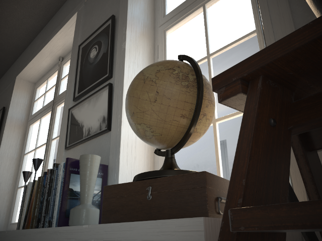
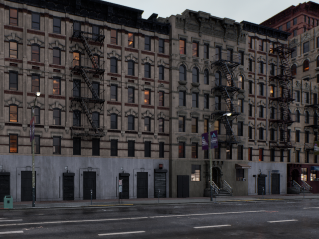
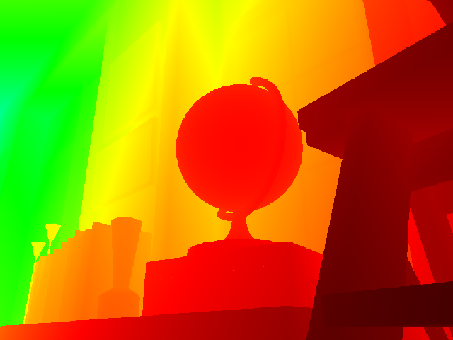
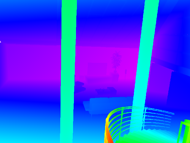
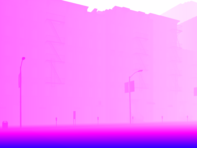
Give your depth estimation a fancy new colormap! Here you'll find an implementation of a bijective metric depth $\leftrightarrow$ RGB mapping along a 3D Hilbert cube walk, as used in the Vision Banana 🍌 paper [1].
 |
 |
 |
 |
 |
 |
📦 Installation
From PyPI:
pip install hilbertmap
From source:
git clone https://github.com/massimilianoviola/hilbertmap
cd hilbertmap
pip install -e .
🛠️ Usage
Direct encoding/decoding
import numpy as np
from hilbertmap import depth_to_rgb, rgb_to_depth

depth = np.load("depth.npy")          # (H, W) float meters
rgb   = depth_to_rgb(depth)           # (H, W, 3) float in [0, 1]
back  = rgb_to_depth(rgb)             # (H, W) recovered meters
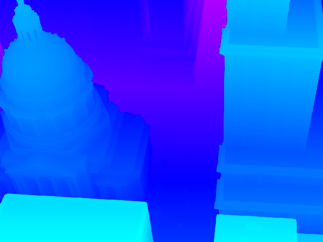
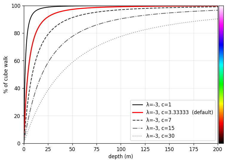
Because the utility of accurate metric depth for nearby image content is generally higher than that of distant content, the default parameters $\lambda = -3$, $c = 10/3$ make the cube walk most sensitive in the first few meters and saturate beyond ~40 m. This behavior can be tuned by changing the parameters to get more meaningful color variation on deep outdoor scenes.
rgb = depth_to_rgb(depth, lam=-4.0, c=120.0) # tuned for long-range outdoor scene
 |
 |
To swap the Barron transform (see explanation below) for a different normalization (linear, log, etc.), use the cube walk primitives directly. hm.walk maps a scalar in $[0, 1]$ to RGB along the cube path, and hm.project is its inverse:
f    = np.clip((depth - vmin) / (vmax - vmin), 0.0, 1.0)  # any forward map from [0, inf) to [0, 1]
rgb  = hm.walk(f)

back = vmin + (vmax - vmin) * hm.project(rgb)             # invert to recover depth
Visualization with matplotlib
import matplotlib.pyplot as plt
import hilbertmap as hm

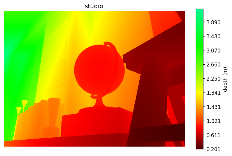
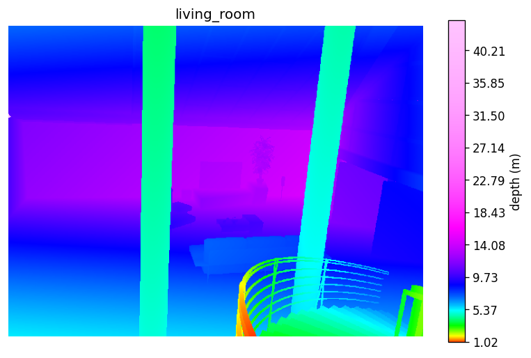
im = plt.imshow(depth, cmap=hm.cmap(), norm=hm.Norm())
hm.colorbar(im, label="depth (m)")
plt.show()
hm.Norm applies the fixed power transform (same depth $\to$ same color across images). With this, hm.colorbar spans only the cmap subset the data actually covers.
 |
 |
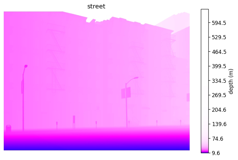 |
In addition, transform params can be tuned as in direct encoding:
im = plt.imshow(depth, cmap=hm.cmap(), norm=hm.Norm(lam=-4.0, c=120.0))  # global, long-range outdoor
hm.colorbar(im, label="depth (m)")
plt.show()
Note that passing vmin / vmax to hm.Norm does not rescale the mapping, only the displayed colorbar range:
im = plt.imshow(depth, cmap=hm.cmap(), norm=hm.Norm(vmin=2.0, vmax=10.0))  # same global mapping, colorbar rescaled
hm.colorbar(im, label="depth (m)")  # <- this now shows [2, 10]
plt.show()
For per-image rescaling without the power transform, pair hm.cmap() with a standard matplotlib normalizer or simply omit it. This is the default behavior of other matplotlib colormaps.
Omit the normalizer to autoscale linearly to the data's min and max:
im = plt.imshow(depth, cmap=hm.cmap())  # linear, autoscaled to min/max, covering full cmap from black to white
hm.colorbar(im, label="depth (m)")
plt.show()
Or pass vmin and vmax for a fixed range:
im = plt.imshow(depth, cmap=hm.cmap(), vmin=0.0, vmax=80.0)               # linear, fixed range
# im = plt.imshow(depth, cmap=hm.cmap(), norm=plt.Normalize(0.0, 80.0))   # equivalent
hm.colorbar(im, label="depth (m)")
plt.show()
🧭 How it works
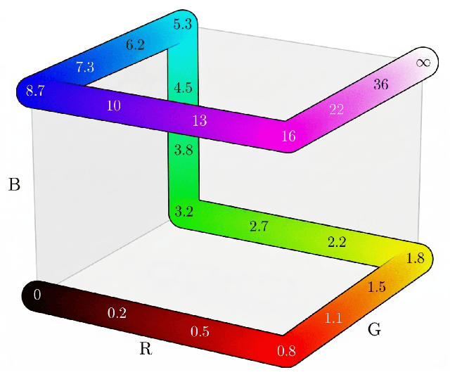
The seven-edge Hamiltonian path on the RGB cube (left) carries depth values from black at zero to white at infinity. The shape parameters $\lambda$ and $c$ produce different saturation curves (right) that decide how much depth lives on each segment of the walk.
| Cube walk | Saturation curves |
 |
 |
Unbounded metric depth $d \in [0, \infty)$ is squashed into $[0, 1)$ by a power transform from Barron (2025) [2], with $\lambda < -1$:
$$f(d, \lambda, c) = 1 - \left(1 - \frac{d}{\lambda c}\right)^{\lambda + 1}$$
With defaults $\lambda = -3$, $c = 10/3$ this simplifies to $f(d) = 1 - (1 + d/10)^{-2}$, mapping $d \in [0, \infty)$ to $f \in [0, 1)$, which is then read as the fractional position along the edge walk to land on $\mathrm{RGB} \in [0, 1]^3$. The mapping is a strict bijection, so any RGB encoding can be decoded back to metric depth by projecting onto the nearest edge.
📚 References
- V. Gabeur et al. Vision Banana: Image generators are generalist vision learners. arXiv preprint arXiv:2604.20329, 2026. Project page: https://vision-banana.github.io/.
- J. T. Barron. A power transform. arXiv preprint arXiv:2502.10647, 2025.
1 maintainer

Metadata
1 maintainer
Release files for hilbertmap 0.1.3
For a detailed explanation of source distributions (sdists) and built distributions (wheels), please see the package formats documentation.
Source distribution (sdist)
| File | Size | Uploaded | |
|---|---|---|---|
| hilbertmap-0.1.3.tar.gz | 4.4 MB | Details |
Built distribution (wheel)
| File | Interpreter | ABI | Platform | Reset |
|---|---|---|---|---|
| hilbertmap-0.1.3-py3-none-any.whl | Python 3 | none | any | Details |
Total release size: 4.4 MB
Release files / hilbertmap-0.1.3.tar.gz
| Download URL | hilbertmap-0.1.3.tar.gz |
|---|---|
| Size | 4.4 MB |
| Tags | Source |
|
SHA-256 checksum How to use checksums |
228387d78f344ab4e058974aecc1e54903780e11893bf2f6849100d7560bd01a
|
|
BLAKE2b-256 checksum How to use checksums |
6ef9ce977bfed8543162da8b4ce6e1ec73c866ebf9cc664fd149dc9fac0f517a
|
| Upload date | |
|
Uploaded using Trusted Publishing? What is trusted publishing? |
Yes |
| Uploaded via |
twine/6.1.0 CPython/3.13.12
|
Provenance
Provenance describes where a file came from. On PyPI, provenance is shared via attestations, which provide a verifiable record of the build or publishing details. View details, limitations and caveats.


PyPI Publish Attestation
PyPI verified that this artifact, at this checksum, originated from the publisher listed below.
Signed by GitHub Actions, verified by PyPI on Apr 26, 2026.
Transparency logRelease files / hilbertmap-0.1.3-py3-none-any.whl
| Download URL | hilbertmap-0.1.3-py3-none-any.whl |
|---|---|
| Size | 7.7 kB |
| Tags | Python 3 |
|
SHA-256 checksum How to use checksums |
ae1d5aa99ef03a81448239316d96b73163d4ec22b752b31c166eae170027d6bf
|
|
BLAKE2b-256 checksum How to use checksums |
d971fea064962f4eb693bd430f5f4a6838aeab65024efb8dc20a896b974045fd
|
| Upload date | |
|
Uploaded using Trusted Publishing? What is trusted publishing? |
Yes |
| Uploaded via |
twine/6.1.0 CPython/3.13.12
|
Provenance
Provenance describes where a file came from. On PyPI, provenance is shared via attestations, which provide a verifiable record of the build or publishing details. View details, limitations and caveats.
PyPI Publish Attestation
PyPI verified that this artifact, at this checksum, originated from the publisher listed below.
Signed by GitHub Actions, verified by PyPI on Apr 26, 2026.
Transparency log













