Physical Simulations on Images.

Project description
Image-Physics-Simulation
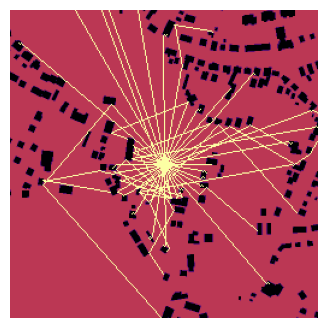
This is a library for 2D Ray-Tracing on an image. For example the Physgen Dataset, see here.
Contents:
- Installation
- Download Example Data
- Library Overview
- Raytracing Computation
- Raytracing Tutorial
- Performance Test
Installation
This repo only need some basic libraries:
numpymatplotlibopencv-pythonscikit-image
You can download / clone this repo and run the example notebook via following Python/Anaconda setup:
conda create -n img-phy-sim python=3.13 pip -y
conda activate img-phy-sim
pip install numpy matplotlib opencv-python ipython jupyter shapely prime_printer datasets==3.6.0 scikit-image
pip install torch torchvision torchaudio --index-url https://download.pytorch.org/whl/cu126
You can also use this repo via Python Package Index (PyPI) as a package:
pip install img-phy-sim
Here the instructions to use the package version of ips and an anconda setup:
conda create -n img-phy-sim python=3.13 pip -y
conda activate img-phy-sim
pip install img-phy-sim
To run the example code you still need:
pip install prime_printer shapely datasets==3.6.0
pip install torch torchvision torchaudio --index-url https://download.pytorch.org/whl/cu126
Download Example Data
You can download Physgen data if wanted via the physgen_dataset.py using following commands:
conda activate img-phy-sim
cd "D:\Informatik\Projekte\Image-Physics-Simulation" && D:
python physgen_dataset.py --output_real_path ./datasets/physgen_train_raw/real --output_osm_path ./datasets/physgen_train_raw/osm --variation sound_reflection --input_type osm --output_type standard --data_mode train
python physgen_dataset.py --output_real_path ./datasets/physgen_test_raw/real --output_osm_path ./datasets/physgen_test_raw/osm --variation sound_reflection --input_type osm --output_type standard --data_mode test
python physgen_dataset.py --output_real_path ./datasets/physgen_val_raw/real --output_osm_path ./datasets/physgen_val_raw/osm --variation sound_reflection --input_type osm --output_type standard --data_mode validation
Library Overview
- Img-Phy-Sim (ips)
ray_tracingget_wall_map: extracting a wall-map from an imagetrace-beam: calculates one raytrace_beams: load an image, extract the wall-map and trace multiple beamsdraw_rays: draw/export the rays as/inside an imageprint_rays_info: get some interesting informations about your rayssave: save your rays as txt fileopen: load your saved rays txt fileget_linear_degree_range: get a range for your beam-directions -> example beams between 0-360 with stepsize 10merge_rays: merge 2 rays to one 'object'
imgopen: load an image via Open-CVsave: save an imageimshow: show an single image (without much features)advanced_imshow: show multiple images with many optionsshow_image_with_line_and_profile: show an image with a red line + the values of the image on this lineplot_image_with_values: plot an image with it's value plotted and averaged to see your image in values
That are not all functions but the ones which should be most useful. Check out the documentation for all functions.
Raytracing Computation
- A map is created which contains the vector of all "walls" (collision objects) in the image as a single degree value. This is done using the
ips.ray_tracing.get_wall_map-function, which internally uses the canny-edge detection algorithm from OpenCV. The whole process is masked to get the edges for the given wall-values. In order to put the degree/direction values into the wall-map, we following theBresenham's line algorithmto go from one point pixel-wise to the end-point of the edge and on the way we put the value of thes epixels and the pixels around, depending of the used thickness. - The
ips.ray_tracing.trace_beam-function goes from pixel to pixel and checks if the pixel-value is a "wall" (collision-object). If yes, a new beam is added using the wall-map to calculate the right direction-vector. To know, which pixel is the next pixel, we use the average vector between the direction vector (the target direction which is available since the beginning of a beam calculation) and a vector pointing to the closest point of the optimal way/vector. Why so complicated? Because we move per pixel and pixel does only know 8 directions, but we want to move more smooth in more directions. The direction vector from the beginning is helpful but will lead every update to the same pixel, because it does not use the information of the current position. THis is bad because so we will move very wrong if going only after the goal vector with our limited step-directions. And so we add the described "to the perfect line"-vector into the calculation weighted a bit less then the real direction (0.5).
The "perfect line" is calculated very easy. At the beginning of a beam we move in small steps (like 0.01) forward towards the target direction, ignoring pixel-wise approach, until we hit with x or y a boundary of the image.
You may have noticed that we use a own and Bresenham's line algorithm for moving in the pixel-space, which have no further reason and we may only use one of them in future.
Raytracing Tutorial
See also the example notebook 👀
In general you need to do:
- Load your Image -> using
ips.img.open - Calculate the Wall-Map -> using
ips.ray_tracing.get_wall_map - Calculate the Beams -> using
ips.img.open - Draw (Export) the Beams -> using
ips.img.open
Using this lib, this is reduced to:
- Calculate the Beams (including Wall-Map and loading your Image) -> using
ips.img.open - Draw (Export) the Beams -> using
ips.img.open
See this example:
rays = ips.ray_tracing.trace_beams(rel_position=[0.5, 0.5],
                                   img_src=img_src,
                                   directions_in_degree=ips.ray_tracing.get_linear_degree_range(step_size=10),
                                   wall_values=None,
                                   wall_thickness=1,
                                   img_border_also_collide=False,
                                   reflexion_order=1,
                                   should_scale_rays=True,
                                   should_scale_img=True)
ips.ray_tracing.print_rays_info(rays)

ray_img = ips.ray_tracing.draw_rays(rays, detail_draw=False,
                                    output_format="single_image",
                                    img_background=img, ray_value=2, ray_thickness=1,
                                    img_shape=(256, 256), dtype=float, standard_value=0,
                                    should_scale_rays_to_image=True, original_max_width=None, original_max_height=None)
ips.img.imshow(ray_img, size=5)
Rays structure:
The Raytracing result is a list of rays, where every ray can consist of multiple beams which comes from reflections. One beam is a list of multiple points, where the first point is the start point and the last element is the end point.
Example:
[
    [[start-point, ..., end-point], [start-point, ..., end-point]],  # one reflection
    [[start-point, ..., end-point]],  # no reflection
    # ...
]
Now let's go step by step how to apply ray-tracing to your image.
1. Analyzing your image
First it is important you know the values of your image and which values should consider an object for collision. For that use the tools given with this package:
img = ips.img.open(src=img_src, should_scale=False, should_print=True)
ips.img.imshow(img, size=4, axis_off=False)
ips.img.show_image_with_line_and_profile(imgs=[img], axis='row', index=None, titles=None, figsize=(10, 8));
If you see super small values then you might tried to scale your already scaled image.
2. Get the Collision Ready
Next it is helpful to check if your collision is ready by running the wall-map by yourself (later you will use the wrapper, but here you can find the right params).
wall_map = ips.ray_tracing.get_wall_map(img, wall_values=None, thickness=0)
ips.img.imshow(wall_map, size=4, axis_off=False)
ips.img.show_image_with_line_and_profile(imgs=[wall_map], axis='row', index=None, titles=None, figsize=(10, 8));
You can give wall_values a list of values, which you want to collide with.
3. Let's start tracing the rays!
Now everything should be ready for tracing the rays. The following code include loading your image and creating the wall-map.
rays = ips.ray_tracing.trace_beams(rel_position=[0.5, 0.5],
                                   img_src="./my_image.png",
                                   directions_in_degree=ips.ray_tracing.get_linear_degree_range(start=0, stop=360, step_size=10),
                                   wall_values=[0.0],
                                   wall_thickness=0,
                                   img_border_also_collide=False,
                                   reflexion_order=1,
                                   should_scale_rays=True,
                                   should_scale_img=True)
ips.ray_tracing.print_rays_info(rays)
Following features are included:
- Setting custom startposition for raytracing
- Adding custom beam shooting positions in degree (where 0° is the east/right of the image and 90° is south/bottom and so on)
- Setting reflexion order (how many maxium reflexions should be calculated)
- Setting if the border of the image should be reflective or not
- And setting if the input image should be scaled and if the rays itself should be scaled
- You can also set the "wall" object values, which should get detected as objects with collision. If set to None, the programm will find all clear edges.
- Setting if the rays should be in 0.0-1.0 range or the real image range
- Whether to scale the image or not
4. Export your rays
At the end you might want to use your rays in an image. We provide you with a draw/export function with many flexibility.
Features are:
- Custom value of ray-traces
- Thickness of ray-traces
- Drawing on empty image or an existing image
- Given image-shape, dtype and fill-value (standard-value)
- Scaling rays to the given image
- Different Format Types
- One Image ->
single_image - Multiple Images (each ray on one image) ->
multiple_images - One Image and each channel is one ray ->
channels
- One Image ->
- Showing only the reflexions
- Give different values for different reflexion orders
ray_img = ips.ray_tracing.draw_rays(rays, detail_draw=False,
                                    output_format="single_image",
                                    img_background=None, ray_value=2, ray_thickness=1,
                                    img_shape=(256, 256), dtype=float, standard_value=0,
                                    should_scale_rays_to_image=False, original_max_width=None, original_max_height=None,
                                    show_only_reflections=False)
ips.img.imshow(ray_img, size=4)
I hope this little tutorial could be helpful. Good luck with your project <3
Performance Test
Executed with 50 random images.
Standard Settings were:
- test_amount=50
- step_size=10
- reflexion_order=3
- ray_scaling=True
- detail_draw=False
- output_format="channels"
Investigated Factors:
Ray Amount(step_size)Scaling of Rays(ray_scaling)Reflexion Order(reflexion_order)Detail Drawing of Rays(detail_draw)
Experiment 1: Ray Amount
Number of experiments: 4

            avg_time            : mean=16.0064, std=23.6257, min=0.5744, max=56.7918, rel_change=351.22%
            median_time         : mean=15.4329, std=22.7908, min=0.5546, max=54.7799, rel_change=351.36%
            var_time            : mean=17.1176, std=29.2774, min=0.0076, max=67.8259, rel_change=396.19%
            avg_compute_time    : mean=15.1070, std=22.2322, min=0.5529, max=53.4815, rel_change=350.36%
            median_compute_time : mean=14.5613, std=21.4404, min=0.5346, max=51.5723, rel_change=350.50%
            var_compute_time    : mean=14.7739, std=25.2362, min=0.0074, max=58.4825, rel_change=395.80%
            avg_draw_time       : mean=0.8994, std=1.3940, min=0.0215, max=3.3103, rel_change=365.67%
            median_draw_time    : mean=0.8373, std=1.2914, min=0.0207, max=3.0705, rel_change=364.22%
            var_draw_time       : mean=0.1525, std=0.2639, min=0.0000, max=0.6096, rel_change=399.67%

Overall trend in avg_time: increasing (1.7306e+01 change per experiment)
Conclusion: Performance changes significantly across experiments.
Experiment 2: Ray Scaling
Number of experiments: 2

            avg_time            : mean=0.5744, std=0.0078, min=0.5666, max=0.5823, rel_change=2.73%
            median_time         : mean=0.5558, std=0.0080, min=0.5478, max=0.5637, rel_change=2.86%
            var_time            : mean=0.0078, std=0.0000, min=0.0078, max=0.0078, rel_change=0.16%
            avg_compute_time    : mean=0.5581, std=0.0024, min=0.5557, max=0.5605, rel_change=0.86%
            median_compute_time : mean=0.5398, std=0.0026, min=0.5372, max=0.5423, rel_change=0.95%
            var_compute_time    : mean=0.0075, std=0.0000, min=0.0075, max=0.0075, rel_change=0.13%
            avg_draw_time       : mean=0.0163, std=0.0055, min=0.0108, max=0.0218, rel_change=66.90%
            median_draw_time    : mean=0.0160, std=0.0053, min=0.0106, max=0.0213, rel_change=66.86%
            var_draw_time       : mean=0.0000, std=0.0000, min=0.0000, max=0.0000, rel_change=67.83%

Overall trend in avg_time: decreasing (-1.5690e-02 change per experiment)
Conclusion: Performance changes slightly across experiments.
Experiment 3: Reflexion Order
Number of experiments: 6

            avg_time            : mean=0.9300, std=0.7354, min=0.3231, max=2.4409, rel_change=227.71%
            median_time         : mean=0.8502, std=0.6128, min=0.3253, max=2.0917, rel_change=207.76%
            var_time            : mean=0.4635, std=0.9329, min=0.0002, max=2.5421, rel_change=548.45%
            avg_compute_time    : mean=0.9014, std=0.7194, min=0.3088, max=2.3798, rel_change=229.74%
            median_compute_time : mean=0.8241, std=0.6002, min=0.3108, max=2.0401, rel_change=209.83%
            var_compute_time    : mean=0.4449, std=0.8953, min=0.0002, max=2.4396, rel_change=548.32%
            avg_draw_time       : mean=0.0286, std=0.0160, min=0.0143, max=0.0611, rel_change=163.74%
            median_draw_time    : mean=0.0266, std=0.0129, min=0.0144, max=0.0521, rel_change=142.21%
            var_draw_time       : mean=0.0002, std=0.0004, min=0.0000, max=0.0011, rel_change=550.06%

Overall trend in avg_time: increasing (3.7365e-01 change per experiment)
Conclusion: Performance changes significantly across experiments.
Experiment 4: Detail Draw
Number of experiments: 2

            avg_time            : mean=0.6282, std=0.0515, min=0.5767, max=0.6796, rel_change=16.39%
            median_time         : mean=0.6101, std=0.0507, min=0.5593, max=0.6608, rel_change=16.63%
            var_time            : mean=0.0115, std=0.0040, min=0.0074, max=0.0155, rel_change=70.54%
            avg_compute_time    : mean=0.5572, std=0.0020, min=0.5552, max=0.5592, rel_change=0.70%
            median_compute_time : mean=0.5430, std=0.0047, min=0.5383, max=0.5478, rel_change=1.75%
            var_compute_time    : mean=0.0074, std=0.0002, min=0.0072, max=0.0076, rel_change=5.32%
            avg_draw_time       : mean=0.0709, std=0.0495, min=0.0214, max=0.1204, rel_change=139.55%
            median_draw_time    : mean=0.0663, std=0.0454, min=0.0209, max=0.1117, rel_change=137.05%
            var_draw_time       : mean=0.0011, std=0.0011, min=0.0000, max=0.0022, rel_change=199.31%

Overall trend in avg_time: increasing (1.0292e-01 change per experiment)
Conclusion: Performance changes slightly across experiments.
Summary:
The Stepsize/amount of rays have the biggest impact on the performance. The other parameters have rather a small impact.
| Experiment | Number of Experiments | avg_time (mean ± std) | avg_compute_time (mean ± std) | avg_draw_time (mean ± std) | rel_change (avg_time) | Trend | Conclusion |
|---|---|---|---|---|---|---|---|
| 1. Ray Amount | 4 | 16.01 ± 23.63 s | 15.11 ± 22.23 s | 0.90 ± 1.39 s | 351.22 % | Increasing (+17.31 s/exp) | Performance changes significantly |
| 2. Ray Scaling | 2 | 0.57 ± 0.01 s | 0.56 ± 0.00 s | 0.016 ± 0.006 s | 2.73 % | Decreasing (−0.016 s/exp) | Performance changes slightly |
| 3. Reflection Order | 6 | 0.93 ± 0.74 s | 0.90 ± 0.72 s | 0.029 ± 0.016 s | 227.71 % | Increasing (+0.37 s/exp) | Performance changes significantly |
| 4. Detail Draw | 2 | 0.63 ± 0.05 s | 0.56 ± 0.00 s | 0.071 ± 0.050 s | 16.39 % | Increasing (+0.10 s/exp) | Performance changes slightly |
Release history Release notifications | RSS feed


Download files
Download the file for your platform. If you're not sure which to choose, learn more about installing packages.
Source Distribution
File details
Details for the file img_phy_sim-0.2.tar.gz.
File metadata
- Download URL: img_phy_sim-0.2.tar.gz
- Upload date:
- Size: 31.2 kB
- Tags: Source
- Uploaded using Trusted Publishing? No
- Uploaded via: twine/6.1.0 CPython/3.12.7
File hashes
| Algorithm | Hash digest | |
|---|---|---|
| SHA256 |
3d2fd7f5c315345d1cccfe8e972cb25b9eae1bca1fc94932780ba064dccd5c9f
|
|
| MD5 |
2b51009b766e1099ed059785b86a0d5d
|
|
| BLAKE2b-256 |
55a70c37d54b40fece6bc69ef667b4c4cdbd34f1dd51a5fcada0dc1bb89bee4a
|


