
IsoTracks
Isoform models, reads with poly(A) tails, RNA modifications, coverage and gene fusions from IsoForge long-read RNA-seq results, one gene per figure.
Give IsoTracks an IsoForge run:
isotracks plot --gene SAT1 --isoforge results/project --output figures/SAT1
from isotracks import plot_gene

plot_gene("SAT1", isoforge="results/project", output="figures/SAT1")
results/project is the prefix IsoForge was run with (isoforge annotate --write_bam --o results/project).
Both write figures/SAT1.pdf and figures/SAT1.png at journal column width.
For BAM files of your own, or to name the conditions, add them:
isotracks plot --gene SAT1 --isoforge results/project \
    --bam "Control:Control_1.bam,Control_2.bam;Treated:Treated_1.bam,Treated_2.bam" \
    --output figures/SAT1
plot_gene(
    "SAT1",
    isoforge="results/project",
    bam_files={"Control": ["Control_1.bam", "Control_2.bam"],
               "Treated": ["Treated_1.bam", "Treated_2.bam"]},
    output="figures/SAT1",
)
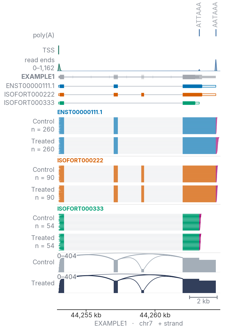
Contents
- Install
- Input
- The figure
- Isoforms and reads
- Views: zoom, close-up, shortened introns, highlights
- Fusion transcripts
- RNA modifications
- Tables
- Appearance
- Command line
- Python API
- Development
- Citation
Install
pip install isotracks
Python 3.10 or later; matplotlib, numpy, pandas, pyarrow, pysam and scipy are installed with it. From source:
git clone https://github.com/MustafaElshani/IsoTracks
cd IsoTracks
pip install .
Input
An IsoForge run
--isoforge (isoforge=) takes the prefix IsoForge was run with (--o results/project), the run's directory,
or any one of its files. IsoTracks reads from it:
| File | Used for |
|---|---|
<prefix>_isoforge.gtf |
the transcript models and the gene's position |
<prefix>_isoforge_read_annot.parquet (or .tsv) |
each read's isoform and poly(A) tail length |
<prefix>_TSS_TES_Clusters/tss_clusters.bed, tes_clusters.bed |
transcription start sites and poly(A) sites |
<prefix>_isoforge_fusion*.parquet |
fusion calls, their transcripts and their reads |
<prefix>_alignments/*.bam |
the alignments, when IsoForge kept them (--write_bam) |
<prefix>_isoforge_sqanti3.bed |
coding extent of the models, when IsoForge_Sqanti3 was run |
Any of these can be given on its own instead (--annotation-gtf, --read-annot, --tss, --polya,
--fusion-table, --bam, --bed); an explicit file takes precedence over the run.
Only whole reads of the transcripts IsoForge reports are drawn (cluster_supported in the read table).
--read-filter all draws every read in the table.
BAM files
The sorted, indexed BAMs IsoForge was given (--bam) or kept (--write_bam). Replicates within a condition are
pooled into one read stack.
-
From the run, samples are grouped as IsoForge groups them: the sample name up to its first underscore is the condition (
Control_1,Control_2→Control). -
With
--bam, conditions are named explicitly:--bam "Control:Control_1.bam,Control_2.bam;Treated:Treated_1.bam,Treated_2.bam" bam_files={"Control": ["Control_1.bam", "Control_2.bam"], "Treated": ["Treated_1.bam", "Treated_2.bam"]}
Poly(A) tail lengths are read from the pt tag of the reads, or from the read annotation when the BAM has none.
Optional
| Option | Adds |
|---|---|
--bed (bed_file=) |
BED12 models with coding extent: CDS is drawn tall and solid, UTRs shorter and hollow. Without it models are drawn from the GTF exons. |
--reference-gtf (reference_gtf=) |
A reference annotation: places genes that are not in the run's GTF, and draws the whole genes of a fusion. |
--modkit, --dmr |
RNA modification tracks. |
The figure
Top to bottom:
| Track | Shows |
|---|---|
| poly(A) | poly(A) sites at the 3′ ends of the drawn isoforms, with their signal hexamer |
| TSS | transcription start sites at their 5′ ends |
| read ends | density of read 5′ and 3′ ends, in reads per 100 bp |
| gene | the drawn isoforms overlaid in grey, with the gene name and direction of transcription |
| isoform models | one row per isoform |
| read stacks | the reads of each isoform, one stack per condition, with poly(A) tails |
| modifications | modified fraction per site, one row per condition |
| differential modification | change in modified fraction between two sample sets |
| coverage | read depth per condition with splice-junction arcs, on one depth axis |
| scale bar and axis | genomic coordinates, chromosome and strand |
- Every figure reads 5′ to 3′ from left to right. A minus-strand gene is drawn with the axis reversed.
- Every read stack has the same height. Its read count is in the gutter (
n = 373). - Coverage is built from the reads of the drawn isoforms. An arc's thickness is the number of reads across that junction.
Isoforms and reads
| Option | Default | Meaning |
|---|---|---|
--min-reads |
5 | least reads per isoform, summed over conditions |
--min-reads-per-condition |
off | least reads per isoform in every condition |
--max-isoforms |
12 | most isoforms drawn, best supported first; 0 for no limit |
--max-reads |
20,000 | most reads drawn per stack; 0 draws all. A thinned stack shows n = 20,000/84,512. |
--coverage-reads |
drawn |
gene builds coverage from every read of the gene |
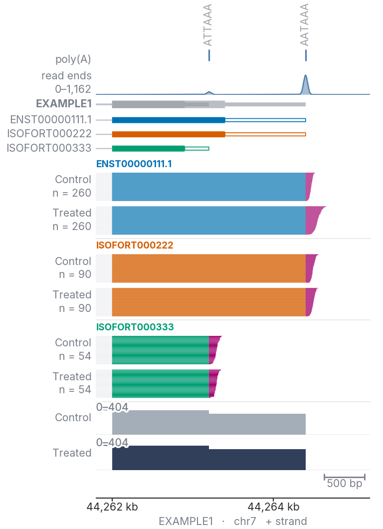
--sort-style |
waterfall |
order of reads within a stack |
waterfall |
diamond |
|---|---|
 |
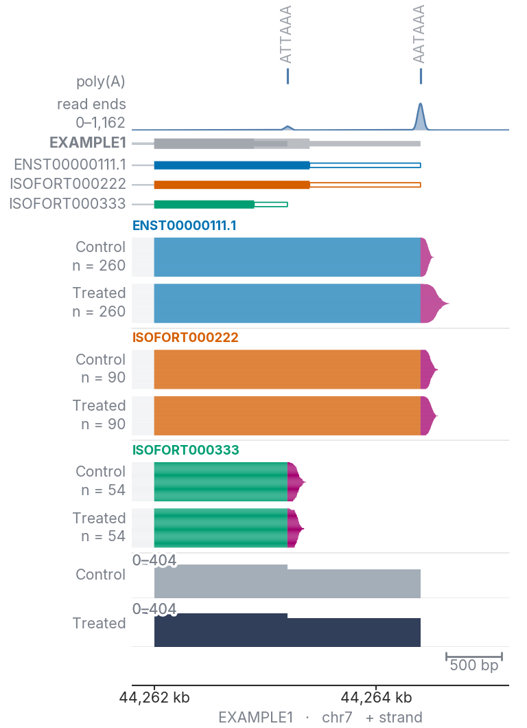 |
| Longest tail at the top. | Longest tail in the middle. |
Views
Zoom
isotracks plot --gene SAT1 ... --zoom last_exon
view.plot(region=view.zoom("last_exon", padding=400))
Targets: first_exon, last_exon, exon_<N>, 5_prime, 3_prime, whole_gene. Exons are numbered 5′ to 3′.
A window reaching the 3′ end is widened to fit the longest poly(A) tail.
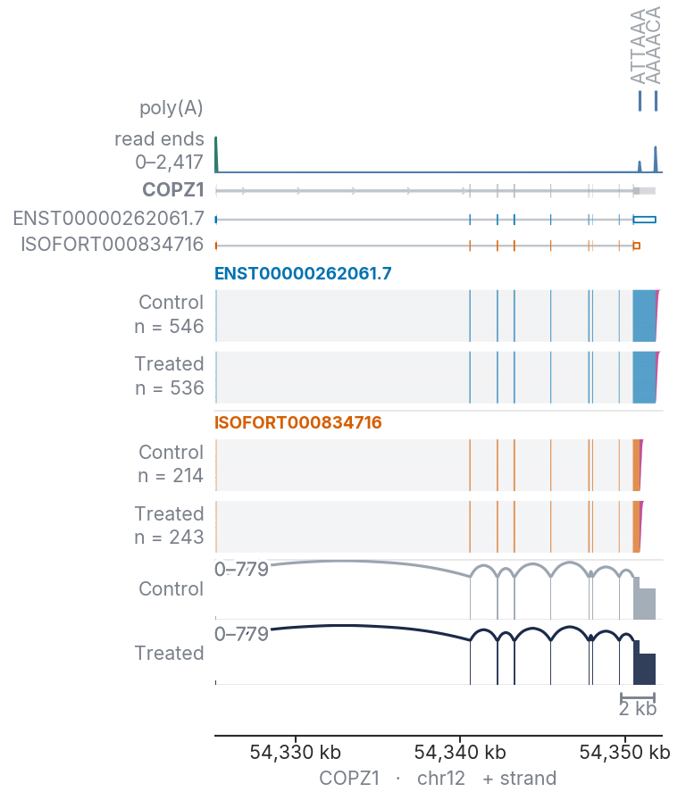
A close-up beside the gene
--detail (detail=) draws a region again beside the whole figure, row for row, at true scale.
| default | --detail last_exon |
|---|---|
 |
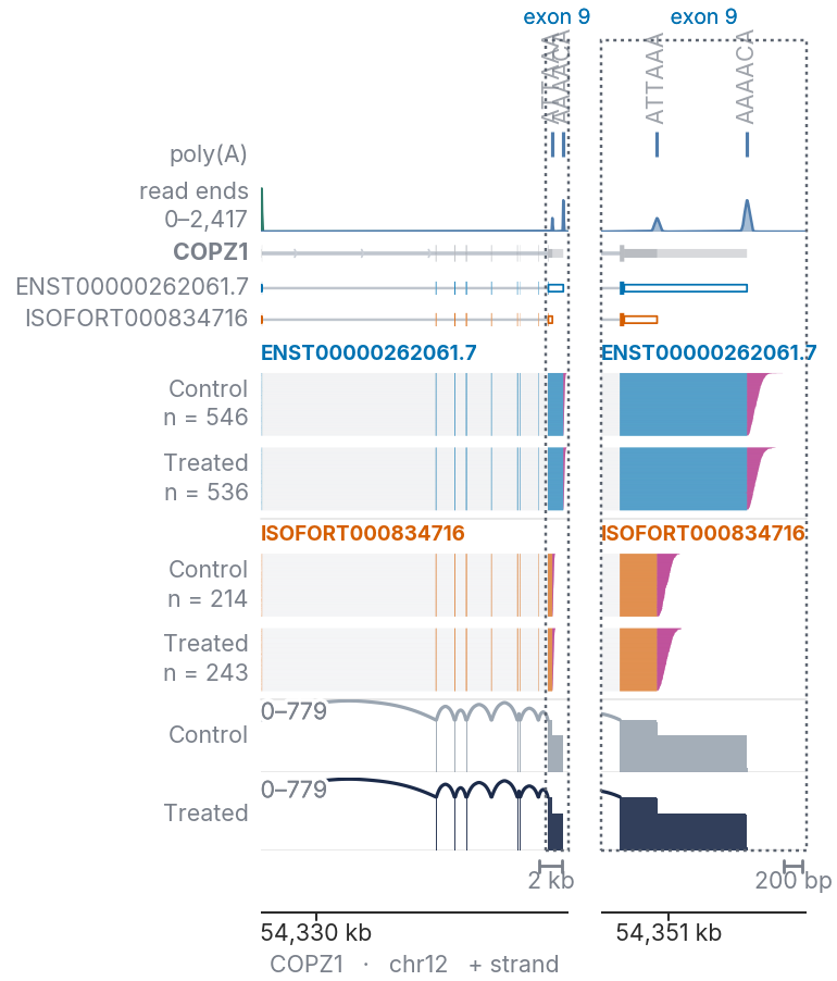 |
It takes last_exon, exon_<N>, 3_utr, junction_<N>, 3_prime, 5_prime or a range. --detail-share sets
the fraction of the width the close-up takes (default 0.4). Depth and read-end density share one scale across
both panels.
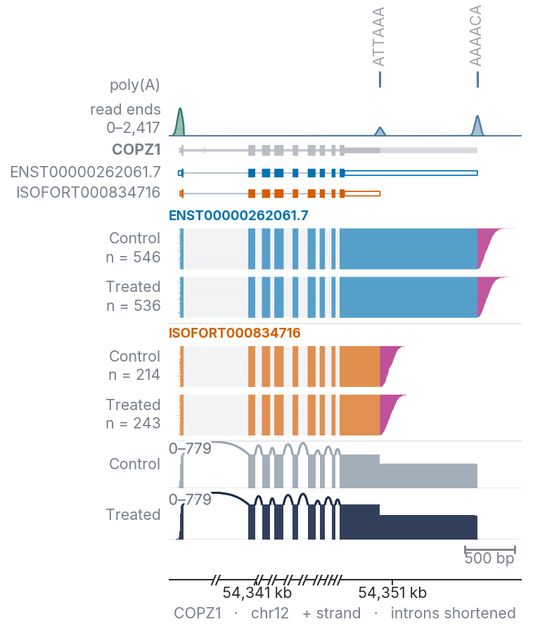
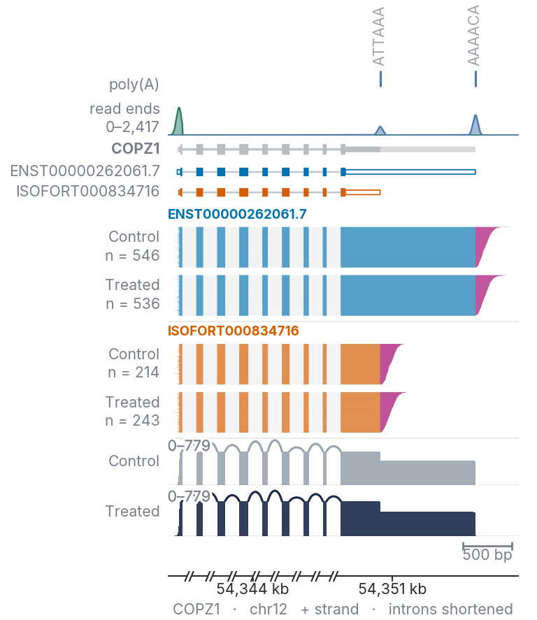
Shortened introns
--introns scaled |
--introns fixed |
|---|---|
 |
 |
Every intron shrunk by one factor; together they take --intron-share of the width (default 0.3). |
Every intron drawn at the same small width. |
Exons, flanks and poly(A) tails stay at true scale. Each shortened intron is marked with // on the axis.
Highlighting a region
--highlight (highlight=) marks regions with a band through every track.
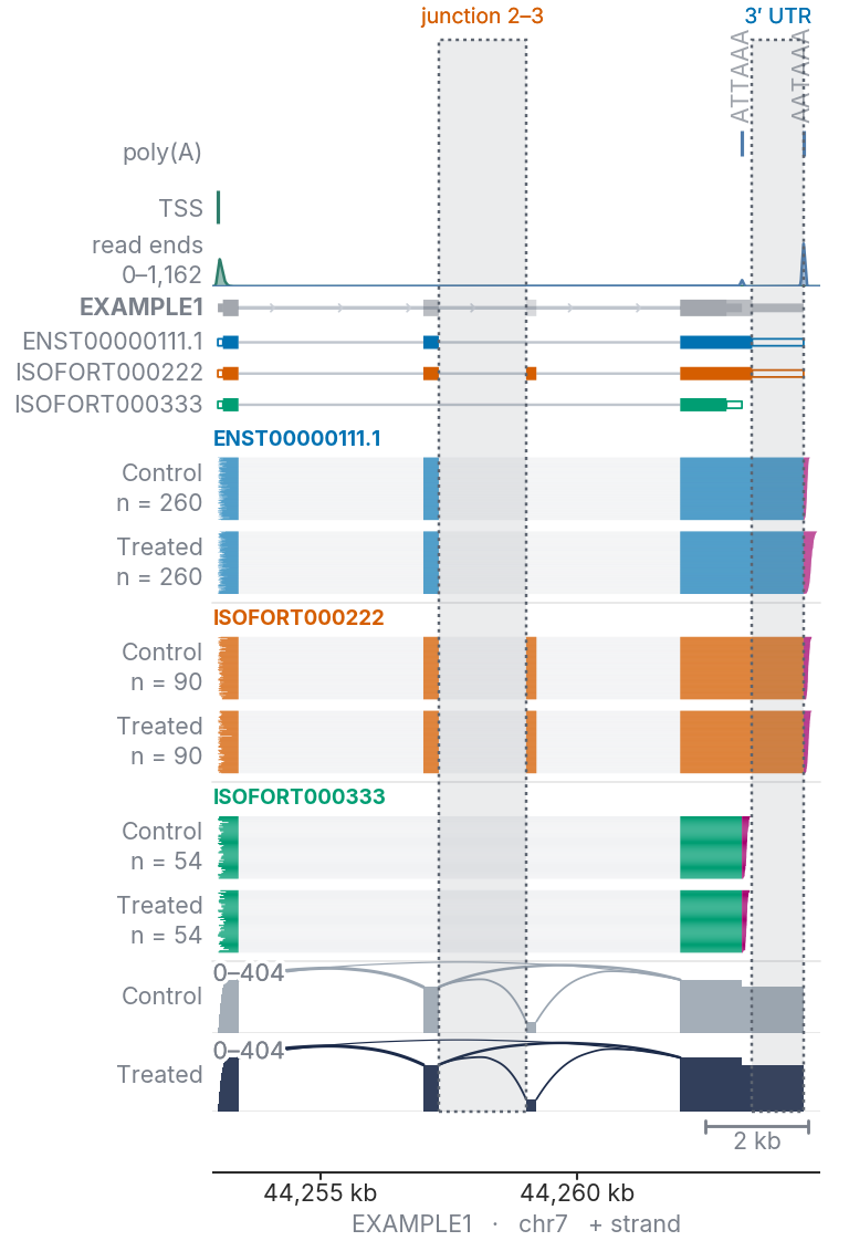
isotracks plot --gene SAT1 ... --highlight junction_2 3_utr
view.plot(highlight=["junction_2", "3_utr:ENST00000111.1"])
view.plot(highlight=(31_950_000, 31_951_000), highlight_style="outline")
| Name | Marks |
|---|---|
exon_<N>, first_exon, last_exon |
one exon, numbered 5′ to 3′ |
intron_<N>, junction_<N> |
the intron between exon N and exon N+1 |
5_utr, 3_utr, cds |
from the coding extent in --bed |
chr22:31,950,000-31,951,000, (start, end) |
that range |
A named region is measured on the isoform with the most exons, or on the one given after a colon
(exon_2:ENST00000111.1). --highlight-style is both (a faint box with a dotted edge), box or outline.
Fusion transcripts
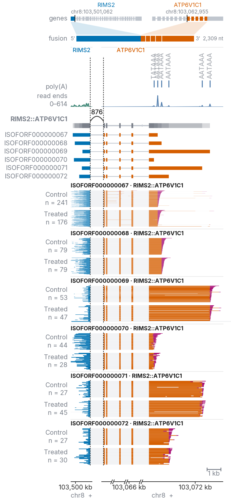
--fusion draws a fusion called by IsoForge, by its genes or its call ID:
isotracks plot --fusion RIMS2::ATP6V1C1 --isoforge results/project \
    --reference-gtf gencode.gtf --output figures/RIMS2_ATP6V1C1
from isotracks import FusionView

view = FusionView("RIMS2::ATP6V1C1", isoforge="results/project", reference_gtf="gencode.gtf")
view.plot(output="figures/RIMS2_ATP6V1C1")
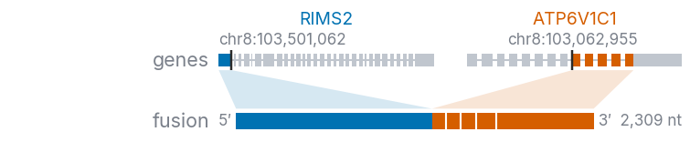
The schematic is drawn at the top of every fusion figure (--no-fusion-schematic leaves it out).
| Row | Shows |
|---|---|
| genes | each partner whole, 5′ to 3′, as its MANE Select isoform. Introns are drawn as equal short gaps; the row is not to scale. The fusion's exons are coloured, the rest of the gene is grey, and each breakpoint is marked with its coordinate. |
| fusion | the fused transcript, exons only, to scale in nucleotides, with its length |
The panels below it follow the gene figure, one panel per partner in transcript order:
| Row | Shows |
|---|---|
| poly(A), TSS | sites at the ends of the fusion transcripts (--polya, --tss, or from --isoforge) |
| read ends | density of the fusion reads' 5′ and 3′ ends, on one scale across the panels |
| fusion gene | the fusion's transcripts overlaid in grey, with an arc and read count over each junction |
| transcripts | one row per fusion transcript, labelled with its IsoForge ID (ISOFORF000000067) |
| read stacks | the reads of each transcript, per condition |
- A dashed line marks each breakpoint through every row.
- Transcripts and reads are joined across the gap between panels: by an intron line where the junction is on splice sites at both ends, and by a dotted line where it is not.
- Introns are shortened within each panel (
--introns scaledis the default for a fusion). - For a fusion of three or more genes, transcripts through every partner are drawn first, then those joining
only some.
--fusion-reads completedraws only the former.
Input. The fusion tables hold every read, so BAMs are optional: they add the poly(A) tails. Samples are
grouped into conditions as for a gene; --conditions "Control:rep1,rep2;Treated:rep3" names the groups without
BAMs. --reference-gtf gives the schematic each partner's whole gene.
A fusion can also be drawn without IsoForge's tables, from a line of breakpoints with its reads found in the
BAMs. A junction is donor>acceptor, the last base kept upstream and the first kept downstream:
FusionView("RIMS2::ATP6V1C1  chr8::chr8  chr8:103501062>chr8:103062955",
           bam_files=bam_files, reference_gtf="gencode.gtf")
RNA modifications
Modification tracks are drawn from modkit pileup bedMethyl files in
genome coordinates, bgzipped and tabix-indexed, one per replicate:
modkit pileup sample.bam sample.bed --ref genome.fa
bgzip sample.bed && tabix -p bed sample.bed.gz
isotracks plot --gene ACTB --isoforge results/project \
    --modkit "Control:Control_1.bed.gz;Treated:Treated_1.bed.gz" --mods a 17802 \
    --output figures/ACTB
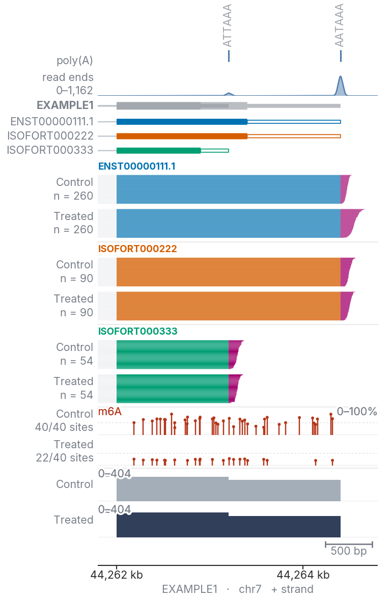
Each lollipop is one site; its height is the modified fraction, from 0 to 100%: reads called modified over reads assessed at that position. Replicates are pooled by summing counts.
| Option | Default | Meaning |
|---|---|---|
--mods |
a,17802 |
codes to draw. Codes joined by commas share a track; separate arguments get a track each. At most three per track. |
--min-mod-coverage |
10 | least reads at a site |
--min-mod-fraction |
0.3 | least modified fraction at a site |
--mod-regions |
exons |
window also draws sites outside the exons of the drawn isoforms |
The gutter reports sites drawn over sites assessed (89/1,933 sites).
| Base | Codes |
|---|---|
| A | a (m6A), 17596 (inosine), 69426 (Am) |
| C | m (5mC), 19228 (Cm) |
| G | 19229 (Gm) |
| U | 17802 (pseudouridine), 19227 (Um) |
Differential modification
--dmr draws the change in modified fraction per site from a modkit dmr pair site table, sorted, bgzipped
and tabix-indexed:
modkit dmr pair -a Control_1.bed.gz -a Control_2.bed.gz -b Treated_1.bed.gz -b Treated_2.bed.gz \
    --ref genome.fa --base A --header -o sites.bed
grep -v '^#' sites.bed | sort -k1,1 -k2,2n | bgzip > sites.bed.gz
tabix -p bed sites.bed.gz
isotracks plot --gene ACTB ... --dmr "Control vs Treated:sites.bed.gz"
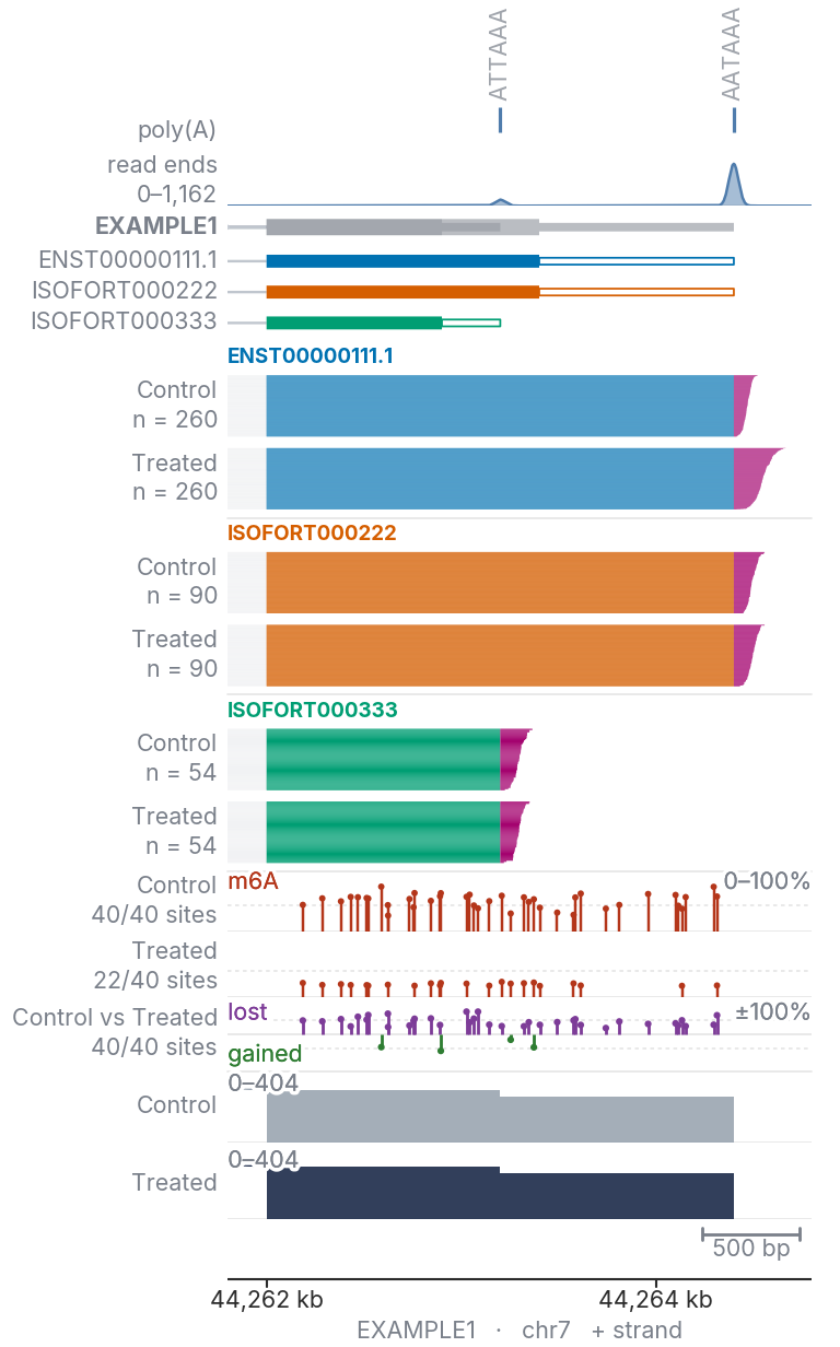
The axis runs from −100% to +100%. modkit's effect size is a − b, so a stem pointing up is a site less
modified in the second sample set, and a stem pointing down one more modified.
| Option | Default | Meaning |
|---|---|---|
--max-diff-pvalue |
0.05 | largest p-value drawn |
--min-diff-effect |
0.2 | smallest change in modified fraction drawn |
--balanced-diff |
off | use modkit's replicate-balanced effect size and p-value |
Tables
Coordinates of a gene's isoforms and exons, 1-based and inclusive:
isotracks info --gene SAT1 --isoforge results/project
isotracks info --gene SAT1 --isoforge results/project --format tsv --exons-table -o exons.tsv
view.print_info()        # the report
view.isoform_table()     # one row per isoform: exons, length, span, reads
view.exons()             # one row per exon
Per-read poly(A) tail lengths:
isotracks polya --gene SAT1 --isoforge results/project -o SAT1_polya.csv
view.polya_table() # gene, transcript_id, condition, sample, read_name, polya_length
Appearance
| Option | Values |
|---|---|
--width |
single (89 mm), onehalf (120), double (183), slide (254), or millimetres |
--readability |
strict, comfortable (default), large |
--roomy |
taller read, coverage and modification tracks; type size is unchanged |
--polya-scale |
base pairs drawn per nucleotide of poly(A) tail (default 1) |
--condition-labels |
display names, "Ctrl:Control,Trt:Treated" |
--condition-colors |
hex colours, "Control:#9AA5B1,Treated:#1B2A49" |
--formats, --dpi |
output formats (default PDF and PNG) and raster resolution (default 600) |
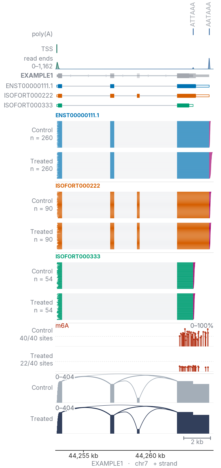
Figures are built at the printed width. Isoform colours are Okabe–Ito. PDF output embeds TrueType fonts and SVG keeps live text.
from isotracks import IsoTracks, Layout, theme

theme.use(width="double", readability="large")
IsoTracks(..., isoform_colors=["#0072B2", "#D55E00"], layout=Layout(read_stack=4.5, coverage=2.0))
Command line
| Command | Does |
|---|---|
isotracks plot |
draw one gene (--gene), region (--region chr:start-end[:strand]) or fusion (--fusion) |
isotracks batch |
draw one figure per gene from a list (--genes genes.txt --outdir figures) |
isotracks info |
report isoform and exon coordinates |
isotracks polya |
write per-read poly(A) tail lengths as CSV |
isotracks index |
index a TSV read annotation by gene; not needed for Parquet |
isotracks <command> --help lists every option.
Python API
from isotracks import IsoTracks

view = IsoTracks(gene_name="SAT1", isoforge="results/project", min_reads_per_condition=5)

view.transcripts()                               # the isoforms drawn
view.plot(output="figures/SAT1")                 # PDF and PNG
view.plot(output="figures/SAT1.svg")             # one format
view.plot(region=view.zoom("last_exon"), sort_style="diamond")
view.plot(detail="last_exon", introns="scaled", highlight="3_utr")
plot_gene(gene, isoforge=..., output=..., **options) builds and draws in one call.
examples/ has a script and a notebook.
Tracks can also be stacked directly:
from isotracks import Canvas
from isotracks.io import CoverageReader

canvas = Canvas()
canvas.add("TranscriptTrack", file_name="models.bed", label="models")
canvas.add("CoverageTrack", reader=CoverageReader(file_names=["a.bam"]), label="depth")
canvas.add("CoordinateAxisTrack")
canvas.render(region=("chr1", 1_000_000, 1_010_000, "+"))
Development
pip install -e ".[dev]"
pytest
The figures in this README are written by the scripts in docs/: make_examples.py from synthetic
data, make_gene_examples.py and make_fusion_example.py from an IsoForge run, and make_logo.py.
src/isotracks/
├── browser.py       IsoTracks, plot_gene: the gene view
├── fusion_view.py   FusionView: the fusion view
├── fusion.py        fusion calls, partners, reads and transcripts
├── isoforge.py      the files of an IsoForge run
├── annotation.py    GTF, read annotation and BED12
├── canvas.py        the figure: tracks in rows, in one or more panels
├── theme.py         widths, type sizes and colours
├── layout.py        track heights
├── cli.py           the isotracks command
├── io/              readers for alignments, features, sites and modifications
└── tracks/          one module per track type
Citation
IsoTracks is a companion tool of IsoForge. The IsoForge manuscript is in preparation. Until it is out, please cite the IsoForge repository:
Elshani M, Zhang Y, Harrison DJ. IsoForge, version 1.0.0. https://github.com/MustafaElshani/IsoForge
License
MIT
1 maintainer

Metadata
1 maintainer
Release files for isotracks 1.0.0
For a detailed explanation of source distributions (sdists) and built distributions (wheels), please see the package formats documentation.
Source distribution (sdist)
| File | Size | Uploaded | |
|---|---|---|---|
| isotracks-1.0.0.tar.gz | 160.7 kB | Details |
Built distribution (wheel)
| File | Interpreter | ABI | Platform | Reset |
|---|---|---|---|---|
| isotracks-1.0.0-py3-none-any.whl | Python 3 | none | any | Details |
Total release size: 291.9 kB
Release files / isotracks-1.0.0.tar.gz
| Download URL | isotracks-1.0.0.tar.gz |
|---|---|
| Size | 160.7 kB |
| Tags | Source |
|
SHA-256 checksum How to use checksums |
4f6ab1823f91c453163460e3d7e0aa3d844944180a36896195dac13e87338dac
|
|
BLAKE2b-256 checksum How to use checksums |
cb03c0a37bd152fb2dd15f1fb2b5eaee7e3d0c582f9d06a5f0723dc986963be4
|
| Upload date | |
|
Uploaded using Trusted Publishing? What is trusted publishing? |
Yes |
| Uploaded via |
twine/7.0.0 CPython/3.13.14
|
Provenance
Provenance describes where a file came from. On PyPI, provenance is shared via attestations, which provide a verifiable record of the build or publishing details. View details, limitations and caveats.


PyPI Publish Attestation
PyPI verified that this artifact, at this checksum, originated from the publisher listed below.
Signed by GitHub Actions, verified by PyPI on Oct 10, 2026.
Transparency logRelease files / isotracks-1.0.0-py3-none-any.whl
| Download URL | isotracks-1.0.0-py3-none-any.whl |
|---|---|
| Size | 131.2 kB |
| Tags | Python 3 |
|
SHA-256 checksum How to use checksums |
735acd894fa59ef6302c51eae5de8a6138177b9e31bcc5349f5748432946b4fe
|
|
BLAKE2b-256 checksum How to use checksums |
b623debf8c22befcdcc314f8442a59e5d393d94539c1ca6fb39d1fee71c68797
|
| Upload date | |
|
Uploaded using Trusted Publishing? What is trusted publishing? |
Yes |
| Uploaded via |
twine/7.0.0 CPython/3.13.14
|
Provenance
Provenance describes where a file came from. On PyPI, provenance is shared via attestations, which provide a verifiable record of the build or publishing details. View details, limitations and caveats.
PyPI Publish Attestation
PyPI verified that this artifact, at this checksum, originated from the publisher listed below.
Signed by GitHub Actions, verified by PyPI on Oct 10, 2026.
Transparency log












