Analytics for quants
Verified details
These details have been verified by PyPIProject links
GitHub Statistics
Maintainers


Project description
jQuantStats: Portfolio Analytics for Quants


📊 Overview
jQuantStats is a Python library for portfolio analytics that helps quants and portfolio managers understand their performance through in-depth analytics and risk metrics. It provides tools for calculating various performance metrics and visualizing portfolio performance using interactive Plotly charts.
The library is inspired by QuantStats, but focuses on providing a clean, modern API with enhanced visualization capabilities. Key improvements include:
- Polars-native design with zero pandas runtime dependency
- Modern interactive visualizations using Plotly
- Comprehensive test coverage with pytest
- Clean, well-documented API
- Efficient data processing with polars
⚡ jQuantStats vs QuantStats
| Feature | jQuantStats | QuantStats |
|---|---|---|
| DataFrame engine | Polars (zero pandas at runtime) | pandas |
| Visualisation | Interactive Plotly charts | Static matplotlib / seaborn |
| Input format | polars.DataFrame |
pandas.Series / pandas.DataFrame |
| Entry point — positions | Portfolio.from_cash_position(prices, cash_position, aum) |
— |
| Entry point — returns | Data.from_returns(returns, benchmark) |
qs.reports.full(returns) |
| HTML report | portfolio.report.full() |
qs.reports.html(returns) |
| Snapshot chart | data.plots.plot_snapshot() |
qs.plots.snapshot(returns) |
| Sharpe ratio | data.stats.sharpe() |
qs.stats.sharpe(returns) |
| Sortino ratio | data.stats.sortino() |
qs.stats.sortino(returns) |
| Max drawdown | data.stats.max_drawdown() |
qs.stats.max_drawdown(returns) |
| Python version | 3.11+ | 3.7+ |
| Type annotations | Full (py.typed) |
Partial |
| Test coverage | |
— |
✨ Features
- Performance Metrics: Calculate key metrics like Sharpe ratio, Sortino ratio, drawdowns, volatility, and more
- Risk Analysis: Analyze risk through metrics like Value at Risk (VaR), Conditional VaR, and drawdown analysis
- Interactive Visualizations: Create interactive plots for portfolio performance, drawdowns, and return distributions
- Benchmark Comparison: Compare your portfolio performance against benchmarks
- Polars-native: Pure polars at runtime; pandas is not required and not supported as input
🖼️ Dashboard Preview
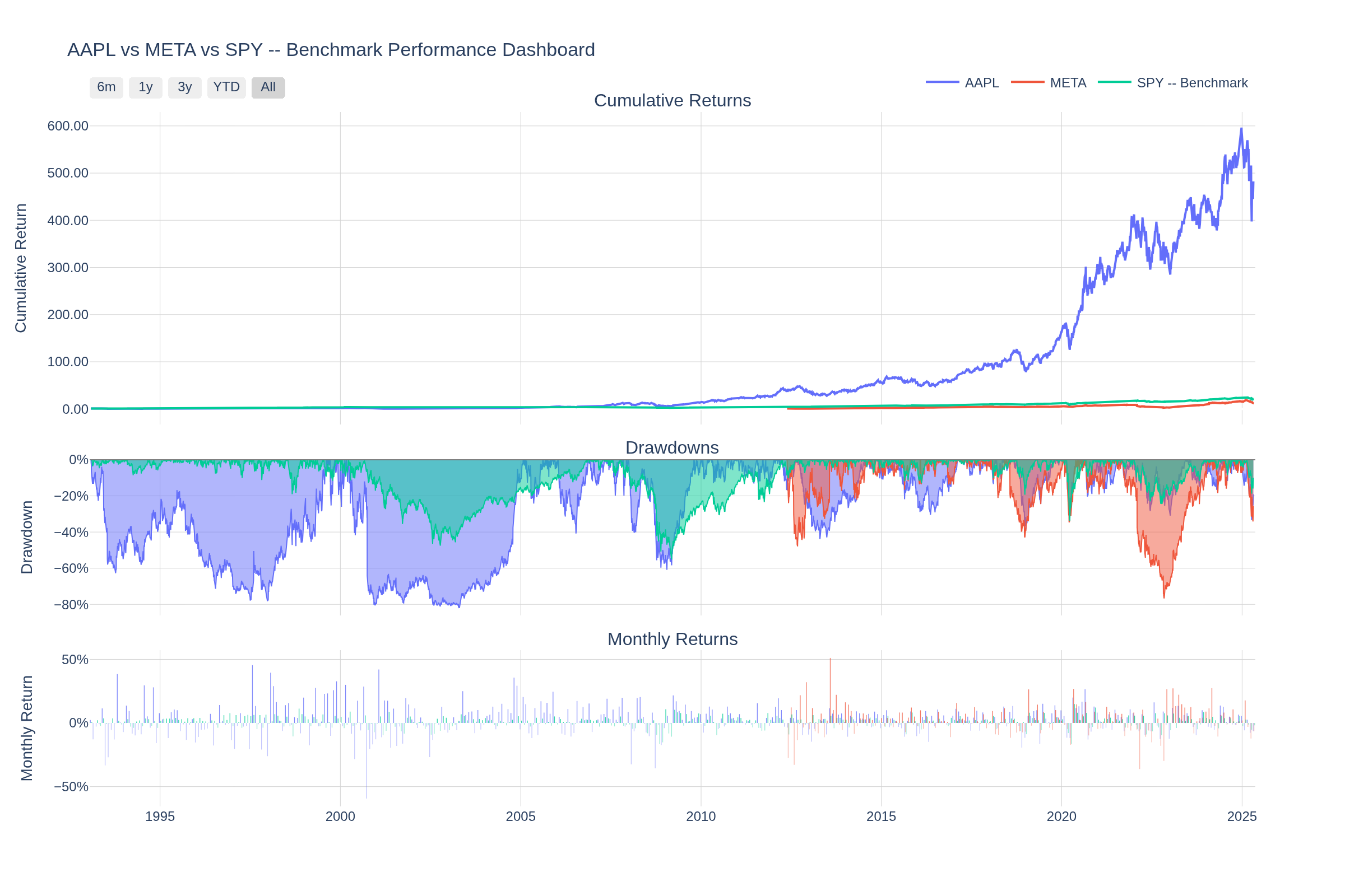
Interactive Plotly dashboard — cumulative returns, drawdowns, and monthly return heatmaps in a single view. Charts are fully interactive (zoom, pan, hover tooltips) when rendered in a browser.
📦 Installation
Using pip:
pip install jquantstats
Using conda (via conda-forge):
conda install -c conda-forge jquantstats
For development:
pip install jquantstats[dev]
🚀 Quick Start
Five lines to your first analytics result:
import polars as pl
from jquantstats import Data

returns = pl.DataFrame({
    "Date": ["2023-01-01", "2023-01-02", "2023-01-03", "2023-01-04", "2023-01-05"],
    "Strategy": [0.01, -0.03, 0.02, -0.01, 0.04],
}).with_columns(pl.col("Date").str.to_date())

benchmark = pl.DataFrame({
    "Date": ["2023-01-01", "2023-01-02", "2023-01-03", "2023-01-04", "2023-01-05"],
    "Benchmark": [0.005, -0.01, 0.008, -0.005, 0.015],
}).with_columns(pl.col("Date").str.to_date())

data = Data.from_returns(returns=returns, benchmark=benchmark)

print(data.stats.sharpe())
# {'Strategy': 4.24, 'Benchmark': 4.94}

print(data.stats.max_drawdown())
# {'Strategy': 0.03, 'Benchmark': 0.01}

fig = data.plots.plot_snapshot(title="Strategy vs Benchmark")
fig.show()  # opens an interactive Plotly chart in your browser
If you have price series and position sizes (recommended):
import polars as pl
from jquantstats import Portfolio

prices = pl.DataFrame({
    "date": ["2023-01-01", "2023-01-02", "2023-01-03"],
    "Asset1": [100.0, 101.0, 99.5],
}).with_columns(pl.col("date").str.to_date())

positions = pl.DataFrame({
    "date": ["2023-01-01", "2023-01-02", "2023-01-03"],
    "Asset1": [1000.0, 1000.0, 1200.0],
}).with_columns(pl.col("date").str.to_date())

pf = Portfolio.from_cash_position(prices=prices, cash_position=positions, aum=1_000_000)

sharpe = pf.stats.sharpe()
fig = pf.plots.snapshot()  # call fig.show() to display
If you already have a returns series:
import polars as pl
from jquantstats import Data

returns = pl.DataFrame({
    "Date": ["2023-01-01", "2023-01-02", "2023-01-03"],
    "Asset1": [0.01, -0.02, 0.03],
    "Asset2": [0.02, 0.01, -0.01]
}).with_columns(pl.col("Date").str.to_date())

data = Data.from_returns(returns=returns)

sharpe = data.stats.sharpe()
fig = data.plots.plot_snapshot(title="Portfolio Performance")  # call fig.show() to display
Risk metrics and drawdown analysis:
import polars as pl
from jquantstats import Data

returns = pl.DataFrame({
    "Date": ["2023-01-01", "2023-01-02", "2023-01-03", "2023-01-04", "2023-01-05"],
    "Strategy": [0.01, -0.03, 0.02, -0.01, 0.04],
}).with_columns(pl.col("Date").str.to_date())

data = Data.from_returns(returns=returns)

sharpe = data.stats.sharpe()
sortino = data.stats.sortino()
max_dd = data.stats.max_drawdown()
vol = data.stats.volatility()
var = data.stats.value_at_risk()
cvar = data.stats.conditional_value_at_risk()
calmar = data.stats.calmar()
win = data.stats.win_rate()
Benchmark comparison:
import polars as pl
from jquantstats import Data

returns = pl.DataFrame({
    "Date": ["2023-01-01", "2023-01-02", "2023-01-03"],
    "Strategy": [0.01, -0.02, 0.03],
}).with_columns(pl.col("Date").str.to_date())

benchmark = pl.DataFrame({
    "Date": ["2023-01-01", "2023-01-02", "2023-01-03"],
    "Benchmark": [0.005, -0.01, 0.015],
}).with_columns(pl.col("Date").str.to_date())

data = Data.from_returns(returns=returns, benchmark=benchmark)

ir = data.stats.information_ratio()
greeks = data.stats.greeks()
alpha = greeks["Strategy"]["alpha"]
beta = greeks["Strategy"]["beta"]
fig = data.plots.plot_snapshot(title="Strategy vs Benchmark")
Generate a full HTML report:
import polars as pl
from jquantstats import Portfolio

prices = pl.DataFrame({
    "date": ["2023-01-01", "2023-01-02", "2023-01-03"],
    "AAPL": [150.0, 152.0, 149.5],
    "MSFT": [250.0, 253.0, 251.0],
}).with_columns(pl.col("date").str.to_date())

positions = pl.DataFrame({
    "date": ["2023-01-01", "2023-01-02", "2023-01-03"],
    "AAPL": [500.0, 500.0, 600.0],
    "MSFT": [300.0, 300.0, 300.0],
}).with_columns(pl.col("date").str.to_date())

pf = Portfolio.from_cash_position(prices=prices, cash_position=positions, aum=1_000_000)

# Save a complete HTML performance report
html = pf.report.to_html()
with open("report.html", "w") as f:
    f.write(html)
🏗️ Architecture
jQuantStats has two layered entry points:
flowchart TD
    A["prices_df + cash_position_df + aum"] --> B["Portfolio.from_cash_position(...)
    NAV compiler"]
    B --> C[".stats  —  full stats suite"]
    B --> D[".plots.snapshot()  —  portfolio plots"]
    B --> E[".report.full()  —  HTML report"]
    B --> F[".data"]

    G["returns_df [+ benchmark_df]"] --> H["Data.from_returns(returns=..., benchmark=...)
    Data object"]
    H --> I[".stats  —  full stats suite"]
    H --> J[".plots.plot_snapshot()  —  snapshot chart"]

    F --> H
Entry point 1 (Portfolio) is for active portfolios where you have
price series and position sizes. It compiles the NAV curve and exposes
the full analytics suite.
Entry point 2 (Data.from_returns) is for arbitrary return streams — e.g.
returns downloaded from a data vendor — with optional benchmark comparison.
The two APIs are layered: portfolio.data returns a Data object, so you
can always drop from a Portfolio into the returns-series API.
📚 Documentation
For detailed documentation, visit jQuantStats Documentation.
🔧 Requirements
- Python 3.11+
- numpy
- polars
- plotly
- scipy
👥 Contributing
Contributions are welcome! Please feel free to submit a Pull Request.
- Fork the repository
- Create your feature branch (
git checkout -b feature/amazing-feature) - Commit your changes (
git commit -m 'Add some amazing feature') - Push to the branch (
git push origin feature/amazing-feature) - Open a Pull Request
📝 Citing
If you use jQuantStats in academic work or research reports, please cite it using the CITATIONS.bib file provided in this repository:
@software{jquantstats,
  author    = {Schmelzer, Thomas},
  title     = {jQuantStats: Portfolio Analytics for Quants},
  url       = {https://github.com/tschm/jquantstats},
  version   = {0.1.1},
  year      = {2026},
  license   = {MIT}
}
⚖️ License
This project is licensed under the MIT License - see the LICENSE file for details.
Project details
Verified details
These details have been verified by PyPIProject links
GitHub Statistics
Maintainers
Release history Release notifications | RSS feed


Download files
Download the file for your platform. If you're not sure which to choose, learn more about installing packages.
Source Distribution
Built Distribution
Filter files by name, interpreter, ABI, and platform.
If you're not sure about the file name format, learn more about wheel file names.
Copy a direct link to the current filters
File details
Details for the file jquantstats-0.3.1.tar.gz.
File metadata
- Download URL: jquantstats-0.3.1.tar.gz
- Upload date:
- Size: 57.0 kB
- Tags: Source
- Uploaded using Trusted Publishing? Yes
- Uploaded via: twine/6.1.0 CPython/3.13.7
File hashes
| Algorithm | Hash digest | |
|---|---|---|
| SHA256 |
9b167483545fa602d7823b1d30c38ca5f0e0ea4f71d84ddf4a6d73abc1f5504f
|
|
| MD5 |
61e4c37d3ae4546ab7074770bef6471b
|
|
| BLAKE2b-256 |
ad0278533d7605bc49dcd032f8e8d72871f02b4eeaf7b91875c24f1f747602df
|
Provenance
The following attestation bundles were made for jquantstats-0.3.1.tar.gz:
Publisher:
rhiza_release.yml on tschm/jquantstats
-
Statement:
-
Statement type:
https://in-toto.io/Statement/v1 -
Predicate type:
https://docs.pypi.org/attestations/publish/v1 -
Subject name:
jquantstats-0.3.1.tar.gz -
Subject digest:
9b167483545fa602d7823b1d30c38ca5f0e0ea4f71d84ddf4a6d73abc1f5504f - Sigstore transparency entry: 1171443225
- Sigstore integration time:
-
Permalink:
tschm/jquantstats@6781a4b1bb0db638d3046d39044a3e00b2a88665 -
Branch / Tag:
refs/tags/v0.3.1 - Owner: https://github.com/tschm
-
Access:
public
-
Token Issuer:
https://token.actions.githubusercontent.com -
Runner Environment:
github-hosted -
Publication workflow:
rhiza_release.yml@6781a4b1bb0db638d3046d39044a3e00b2a88665 -
Trigger Event:
push
-
Statement type:
File details
Details for the file jquantstats-0.3.1-py3-none-any.whl.
File metadata
- Download URL: jquantstats-0.3.1-py3-none-any.whl
- Upload date:
- Size: 62.1 kB
- Tags: Python 3
- Uploaded using Trusted Publishing? Yes
- Uploaded via: twine/6.1.0 CPython/3.13.7
File hashes
| Algorithm | Hash digest | |
|---|---|---|
| SHA256 |
13f183c2f79004ceb6ef025ee7bcd4adf94c3b9f475447f7de863da735571ece
|
|
| MD5 |
5cdcc4605b4671a06f6e74deda2626e2
|
|
| BLAKE2b-256 |
ce7a5181d409fabf7945a472bc5737d8edd90b78c82d6be913c59974a2efc91d
|
Provenance
The following attestation bundles were made for jquantstats-0.3.1-py3-none-any.whl:
Publisher:
rhiza_release.yml on tschm/jquantstats
-
Statement:
-
Statement type:
https://in-toto.io/Statement/v1 -
Predicate type:
https://docs.pypi.org/attestations/publish/v1 -
Subject name:
jquantstats-0.3.1-py3-none-any.whl -
Subject digest:
13f183c2f79004ceb6ef025ee7bcd4adf94c3b9f475447f7de863da735571ece - Sigstore transparency entry: 1171443233
- Sigstore integration time:
-
Permalink:
tschm/jquantstats@6781a4b1bb0db638d3046d39044a3e00b2a88665 -
Branch / Tag:
refs/tags/v0.3.1 - Owner: https://github.com/tschm
-
Access:
public
-
Token Issuer:
https://token.actions.githubusercontent.com -
Runner Environment:
github-hosted -
Publication workflow:
rhiza_release.yml@6781a4b1bb0db638d3046d39044a3e00b2a88665 -
Trigger Event:
push
-
Statement type:


