Analytics for quants
Verified details
These details have been verified by PyPIProject links
GitHub Statistics
Maintainers


Project description
jQuantStats: Portfolio Analytics for Quants


Overview
jQuantStats is a Python library for portfolio analytics that helps quants and portfolio managers understand their strategy performance in depth. It provides two complementary entry points: a Portfolio route that works directly from price and position data, and a Data route for arbitrary return streams. All analytics, visualizations, and HTML reports are available from either entry point.
The library is inspired by QuantStats, but extends it significantly — particularly around position-level analysis that is impossible when you start from a return series alone. Key improvements include:
- Polars-native design with zero pandas runtime dependency
- Modern interactive visualizations using Plotly
- A Portfolio route — the primary entry point — that exposes tools unavailable in QuantStats
- Comprehensive test coverage with pytest
- Clean, fully type-annotated API
The Portfolio Route — Why It Matters
The original QuantStats only accepts a return series. That is convenient but lossy: once you reduce prices and positions to returns, you lose the information needed to answer the questions that matter most in practice.
jQuantStats introduces Portfolio as the primary entry point. You provide the raw
price series and the cash positions your strategy held over time, and the library compiles
the NAV for you. This unlocks a class of analysis tools that simply do not exist in
QuantStats:
Execution-Delay Analysis
Real strategies suffer from execution lag: the signal fires at the close, but the trade
fills the next open, or the next close, or later. A return series hides this completely.
A Portfolio exposes it.
import numpy as np
import polars as pl
from jquantstats import Portfolio

rng = np.random.default_rng(42)
n = 252  # approximately one trading year

prices = pl.DataFrame({
    "date": pl.date_range(pl.date(2020, 1, 2), pl.date(2020, 12, 31), interval="1d", eager=True)[:n],
    "AAPL": (100.0 * np.cumprod(1 + rng.normal(0.0005, 0.015, n))).tolist(),
    "META": (150.0 * np.cumprod(1 + rng.normal(0.0003, 0.018, n))).tolist(),
})

# Allocate $500k to each asset as constant cash positions
positions = prices.select("date").with_columns([
    pl.lit(500_000.0).alias("AAPL"),
    pl.lit(500_000.0).alias("META"),
])

pf = Portfolio.from_cash_position(prices=prices, cash_position=positions, aum=1_000_000)

# Shift all positions forward by one period — simulate T+1 execution
pf_lagged = pf.lag(1)

sharpe_t0 = pf.stats.sharpe()          # ideal (no delay)
sharpe_t1 = pf_lagged.stats.sharpe()   # realistic (T+1 fill)
lag(n) returns a new Portfolio with positions shifted by n periods.
Because every downstream accessor — .stats, .plots, .report — recomputes
on the shifted positions, a single call gives you the full analytics picture
under a different execution assumption.
lead_lag_ir_plot() sweeps the entire range at once and renders it as an
interactive Plotly bar chart:
fig = pf.plots.lead_lag_ir_plot(start=-5, end=10)
# fig.show()  — Sharpe ratio at each lag, from lead-5 to lag+10
This chart immediately answers: how much does a one-day execution delay cost in Sharpe? At what lag does the signal degrade to noise?
Tilt / Timing Attribution
Even without lag analysis, starting from positions lets you decompose performance into two orthogonal sources:
- Tilt — the portfolio with constant average weights (pure allocation skill)
- Timing — the deviation from average weights (pure timing skill)
tilt_pf    = pf.tilt    # constant-weight version of the strategy
timing_pf  = pf.timing  # weight deviations only

tilt_sharpe   = tilt_pf.stats.sharpe()
timing_sharpe = timing_pf.stats.sharpe()

decomp = pf.tilt_timing_decomp  # DataFrame: portfolio | tilt | timing NAVs side by side
Turnover Analytics
turnover         = pf.turnover           # daily one-way turnover as fraction of AUM
turnover_weekly  = pf.turnover_weekly    # weekly aggregate (or 5-period rolling sum)
turnover_summary = pf.turnover_summary() # mean_daily, mean_weekly, turnover_std
turnover         = pf.turnover           # daily one-way turnover as fraction of AUM
turnover_weekly  = pf.turnover_weekly    # weekly aggregate (or 5-period rolling sum)
turnover_summary = pf.turnover_summary() # mean_daily, mean_weekly, turnover_std
Cost Modeling
Two independent cost models, never accidentally combined:
from jquantstats import Portfolio, CostModel

# Model A: per-unit cost (equity, futures tick-size costs)
pf_net = Portfolio.from_cash_position(
    prices=prices, cash_position=positions, aum=1_000_000,
    cost_model=CostModel.per_unit(0.01),
)
net_cost_nav = pf_net.net_cost_nav      # NAV path after deducting position-delta costs

# Model B: turnover-bps cost (macro, fund-of-funds)
pf_bps = Portfolio.from_cash_position(
    prices=prices, cash_position=positions, aum=1_000_000,
    cost_model=CostModel.turnover_bps(5.0),
)
# Sweep Sharpe across 0 → 20 bps in a single call
impact = pf_bps.trading_cost_impact(max_bps=20)
Position Variants
# From unit positions (quantity × price → cash automatically)
units = prices.select("date").with_columns([
    pl.lit(1_000.0).alias("AAPL"),
    pl.lit(500.0).alias("META"),
])
pf = Portfolio.from_position(prices=prices, position=units, aum=1_000_000)

# From risk positions (de-volatized via EWMA, optional vol cap)
risk_units = units
pf = Portfolio.from_risk_position(
    prices=prices, risk_position=risk_units, aum=1_000_000,
    vol_cap=0.20,
)

# Smooth noisy positions with a rolling mean
pf_smooth = pf.smoothed_holding(n=5)
jQuantStats vs QuantStats
| Feature | jQuantStats | QuantStats |
|---|---|---|
| DataFrame engine | Polars (zero pandas at runtime) | pandas |
| Visualisation | Interactive Plotly charts | Static matplotlib / seaborn |
| Input format | polars.DataFrame |
pandas.Series / pandas.DataFrame |
| Entry point — positions | Portfolio.from_cash_position(prices, cash_position, aum) |
— |
| Entry point — returns | Data.from_returns(returns, benchmark) |
qs.reports.full(returns) |
| Execution-delay analysis | pf.lag(n) + pf.plots.lead_lag_ir_plot() |
— |
| Tilt / timing decomposition | pf.tilt, pf.timing, pf.tilt_timing_decomp |
— |
| Turnover analytics | pf.turnover, pf.turnover_summary() |
— |
| Cost models | Two models: per-unit and turnover-bps | — |
| Cost-impact sweep | pf.trading_cost_impact(max_bps=20) |
— |
| HTML report | pf.report.to_html() |
qs.reports.html(returns) |
| Snapshot chart | pf.plots.snapshot() |
qs.plots.snapshot(returns) |
| Sharpe ratio | pf.stats.sharpe() |
qs.stats.sharpe(returns) |
| Max drawdown | pf.stats.max_drawdown() |
qs.stats.max_drawdown(returns) |
| Python version | 3.11+ | 3.7+ |
| Type annotations | Full (py.typed) |
Partial |
| Test coverage | |
— |
Dashboard Preview
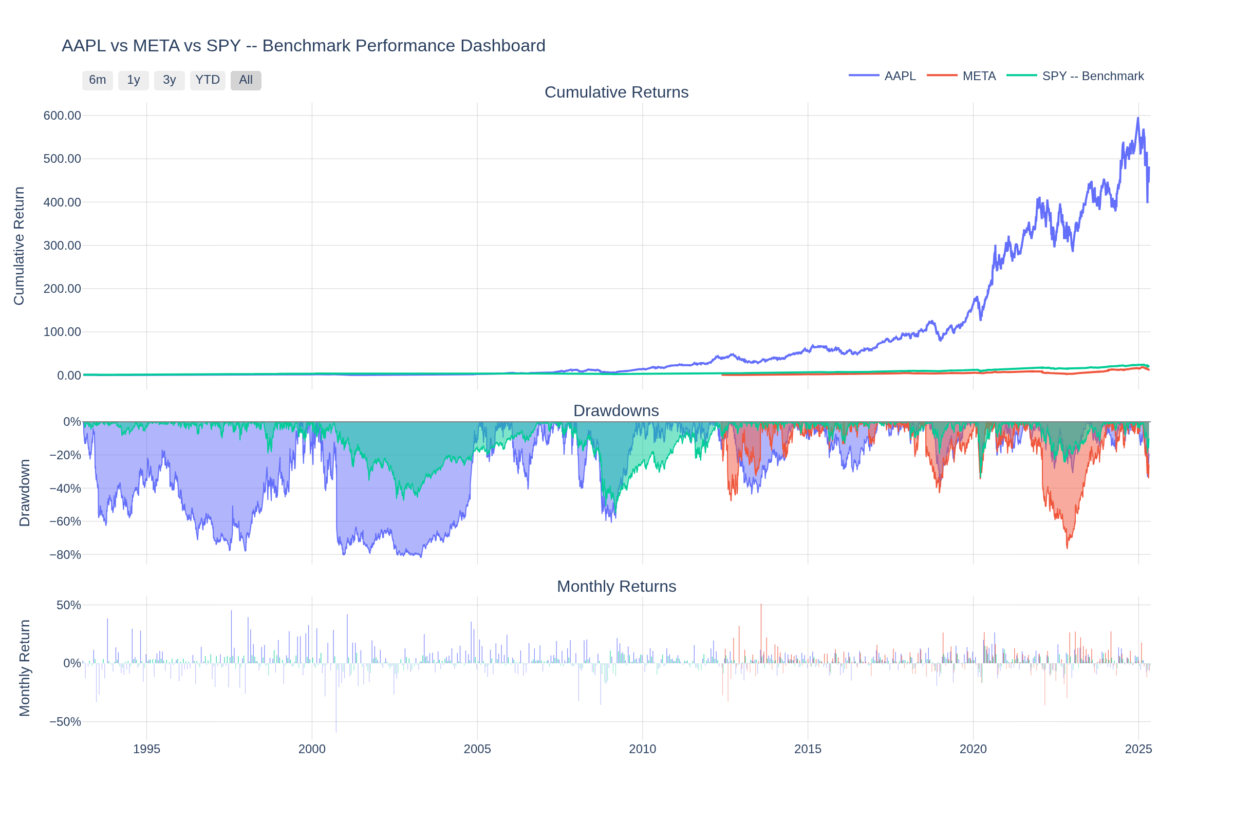
Interactive Plotly dashboard — cumulative returns, drawdowns, and monthly return heatmaps in a single view. Charts are fully interactive (zoom, pan, hover tooltips) when rendered in a browser.
Installation
Using pip:
pip install jquantstats
Using conda (via conda-forge):
conda install -c conda-forge jquantstats
For development:
pip install jquantstats[dev]
Quick Start
Start from prices and positions (recommended)
import polars as pl
from jquantstats import Portfolio

prices = pl.DataFrame({
    "date": ["2023-01-01", "2023-01-02", "2023-01-03"],
    "AAPL": [150.0, 152.0, 149.5],
    "MSFT": [250.0, 253.0, 251.0],
}).with_columns(pl.col("date").str.to_date())

positions = pl.DataFrame({
    "date": ["2023-01-01", "2023-01-02", "2023-01-03"],
    "AAPL": [500.0, 500.0, 600.0],
    "MSFT": [300.0, 300.0, 300.0],
}).with_columns(pl.col("date").str.to_date())

pf = Portfolio.from_cash_position(prices=prices, cash_position=positions, aum=1_000_000)

sharpe = pf.stats.sharpe()
fig = pf.plots.snapshot()   # call fig.show() to display
Compare ideal vs. delayed execution
pf_t0 = pf                # signal executed immediately
pf_t1 = pf.lag(1)         # T+1 execution
pf_t2 = pf.lag(2)         # T+2 execution

sharpe_t0 = pf_t0.stats.sharpe()
sharpe_t1 = pf_t1.stats.sharpe()
sharpe_t2 = pf_t2.stats.sharpe()

# Or visualize the full lead/lag Sharpe profile in one chart
fig = pf.plots.lead_lag_ir_plot(start=-5, end=10)
# fig.show()
Start from a return series
import polars as pl
from jquantstats import Data

returns = pl.DataFrame({
    "Date": ["2023-01-01", "2023-01-02", "2023-01-03", "2023-01-04", "2023-01-05"],
    "Strategy": [0.01, -0.03, 0.02, -0.01, 0.04],
}).with_columns(pl.col("Date").str.to_date())

benchmark = pl.DataFrame({
    "Date": ["2023-01-01", "2023-01-02", "2023-01-03", "2023-01-04", "2023-01-05"],
    "Benchmark": [0.005, -0.01, 0.008, -0.005, 0.015],
}).with_columns(pl.col("Date").str.to_date())

data = Data.from_returns(returns=returns, benchmark=benchmark)

sharpe   = data.stats.sharpe()        # {'Strategy': 4.24, 'Benchmark': 4.94}
max_dd   = data.stats.max_drawdown()  # {'Strategy': 0.03, 'Benchmark': 0.01}
fig      = data.plots.snapshot(title="Strategy vs Benchmark")  # call fig.show() to display
Risk metrics
sharpe  = data.stats.sharpe()
sortino = data.stats.sortino()
max_dd  = data.stats.max_drawdown()
vol     = data.stats.volatility()
var     = data.stats.value_at_risk()
cvar    = data.stats.conditional_value_at_risk()
calmar  = data.stats.calmar()
win     = data.stats.win_rate()
Benchmark comparison
ir     = data.stats.information_ratio()
greeks = data.stats.greeks()
alpha  = greeks["Strategy"]["alpha"]
beta   = greeks["Strategy"]["beta"]
Generate a full HTML report
pf = Portfolio.from_cash_position(prices=prices, cash_position=positions, aum=1_000_000)

html = pf.report.to_html()
with open("report.html", "w") as f:
    f.write(html)
Features
Performance Metrics — Sharpe, Sortino, Calmar, Omega, Treynor, Information Ratio, probabilistic Sharpe/Sortino, smart Sharpe/Sortino, CAGR, GHPR, and more.
Risk Analysis — Value at Risk (VaR), Conditional VaR, drawdown details, max drawdown duration, Ulcer Index, Ulcer Performance Index, risk of ruin.
Win/Loss Statistics — win rate, monthly win rate, profit factor, payoff ratio, consecutive wins/losses, tail ratio, gain-to-pain ratio, outlier win/loss ratios.
Benchmark Analysis — alpha, beta, correlation, tracking error, information ratio, up/down capture ratios, R².
Rolling Analytics — rolling Sharpe, Sortino, volatility, and Greeks with configurable windows.
Portfolio-native (not available in QuantStats):
- Execution-delay analysis via
lag(n)andlead_lag_ir_plot() - Tilt / timing attribution via
tilt,timing,tilt_timing_decomp - Turnover analytics via
turnover,turnover_weekly,turnover_summary() - Cost modeling via
CostModel.per_unit()/CostModel.turnover_bps() - Cost-impact sweep via
trading_cost_impact(max_bps) - Position smoothing via
smoothed_holding(window) - Risk-position entry via
from_risk_position()with EWMA de-volatization
Interactive Visualizations — all charts are Plotly (zoom, pan, hover tooltips, range selectors). Includes portfolio snapshot, lead/lag IR, correlation heatmap, drawdown, rolling returns, rolling volatility, return distribution, monthly heatmap.
HTML Reports — self-contained reports with embedded interactive charts and categorized metric tables, rendered via Jinja2 templates.
Requirements
- Python 3.11+
- numpy
- polars
- plotly
- scipy
Documentation
For detailed documentation, visit jQuantStats Documentation.
Contributing
Contributions are welcome! Please feel free to submit a Pull Request.
- Fork the repository
- Create your feature branch (
git checkout -b feature/amazing-feature) - Commit your changes (
git commit -m 'Add some amazing feature') - Push to the branch (
git push origin feature/amazing-feature) - Open a Pull Request
Citing
If you use jQuantStats in academic work or research reports, please cite it using the CITATIONS.bib file provided in this repository:
@software{jquantstats,
  author    = {Schmelzer, Thomas},
  title     = {jQuantStats: Portfolio Analytics for Quants},
  url       = {https://github.com/jebel-quant/jquantstats},
  version   = {0.4.0},
  year      = {2026},
  license   = {MIT}
}
License
This project is licensed under the MIT License - see the LICENSE file for details.
Project details
Verified details
These details have been verified by PyPIProject links
GitHub Statistics
Maintainers
Release history Release notifications | RSS feed


Download files
Download the file for your platform. If you're not sure which to choose, learn more about installing packages.
Source Distribution
Built Distribution
Filter files by name, interpreter, ABI, and platform.
If you're not sure about the file name format, learn more about wheel file names.
Copy a direct link to the current filters
File details
Details for the file jquantstats-0.6.4.tar.gz.
File metadata
- Download URL: jquantstats-0.6.4.tar.gz
- Upload date:
- Size: 92.2 kB
- Tags: Source
- Uploaded using Trusted Publishing? Yes
- Uploaded via: twine/6.1.0 CPython/3.13.12
File hashes
| Algorithm | Hash digest | |
|---|---|---|
| SHA256 |
c383f1e6dfdb66398a13cba3f718932068b16ee624717b2d1c1a20cd9129738c
|
|
| MD5 |
08aae5799a28eeb36960296448c00764
|
|
| BLAKE2b-256 |
89c1ca904d149294f83116fecaf4864847e0a4d3577203f0c39102a72e5e6d47
|
Provenance
The following attestation bundles were made for jquantstats-0.6.4.tar.gz:
Publisher:
rhiza_release.yml on Jebel-Quant/jquantstats
-
Statement:
-
Statement type:
https://in-toto.io/Statement/v1 -
Predicate type:
https://docs.pypi.org/attestations/publish/v1 -
Subject name:
jquantstats-0.6.4.tar.gz -
Subject digest:
c383f1e6dfdb66398a13cba3f718932068b16ee624717b2d1c1a20cd9129738c - Sigstore transparency entry: 1280659367
- Sigstore integration time:
-
Permalink:
Jebel-Quant/jquantstats@5d509f3ef68aca063fa97cc0a6a5b158dc2886ac -
Branch / Tag:
refs/tags/v0.6.4 - Owner: https://github.com/Jebel-Quant
-
Access:
public
-
Token Issuer:
https://token.actions.githubusercontent.com -
Runner Environment:
github-hosted -
Publication workflow:
rhiza_release.yml@5d509f3ef68aca063fa97cc0a6a5b158dc2886ac -
Trigger Event:
push
-
Statement type:
File details
Details for the file jquantstats-0.6.4-py3-none-any.whl.
File metadata
- Download URL: jquantstats-0.6.4-py3-none-any.whl
- Upload date:
- Size: 104.4 kB
- Tags: Python 3
- Uploaded using Trusted Publishing? Yes
- Uploaded via: twine/6.1.0 CPython/3.13.12
File hashes
| Algorithm | Hash digest | |
|---|---|---|
| SHA256 |
ae6d04948ce8ab5320683678ff0bc3b896a373a76704d46d294c6bcf8bed8917
|
|
| MD5 |
2d9fd2ddbb0c06dd9fd0771e8c23a4d4
|
|
| BLAKE2b-256 |
3d86bc17f0188dc8f8907a1df3b22e6ffcf20069689e22eb9f8137d3b82a2939
|
Provenance
The following attestation bundles were made for jquantstats-0.6.4-py3-none-any.whl:
Publisher:
rhiza_release.yml on Jebel-Quant/jquantstats
-
Statement:
-
Statement type:
https://in-toto.io/Statement/v1 -
Predicate type:
https://docs.pypi.org/attestations/publish/v1 -
Subject name:
jquantstats-0.6.4-py3-none-any.whl -
Subject digest:
ae6d04948ce8ab5320683678ff0bc3b896a373a76704d46d294c6bcf8bed8917 - Sigstore transparency entry: 1280659371
- Sigstore integration time:
-
Permalink:
Jebel-Quant/jquantstats@5d509f3ef68aca063fa97cc0a6a5b158dc2886ac -
Branch / Tag:
refs/tags/v0.6.4 - Owner: https://github.com/Jebel-Quant
-
Access:
public
-
Token Issuer:
https://token.actions.githubusercontent.com -
Runner Environment:
github-hosted -
Publication workflow:
rhiza_release.yml@5d509f3ef68aca063fa97cc0a6a5b158dc2886ac -
Trigger Event:
push
-
Statement type:


