
Topological Centerline SVG Vectorizer for CNC plotters, laser cutters, and CAM software.
Verified details
These details have been verified by PyPIProject links
GitHub Statistics
Maintainers

Project description

KDRAW: Topological Centerline SVG Vectorizer



📸 Visual Documentation & Evidence
💻 Running the Vectorizer
To convert a text image into optimized single-line vectors using custom configuration:
python main.py input.jpg output_centerline.svg --centerline --no-adaptive --morph-close 5 --min-spur 1 --upscale 8 --morph-close 5
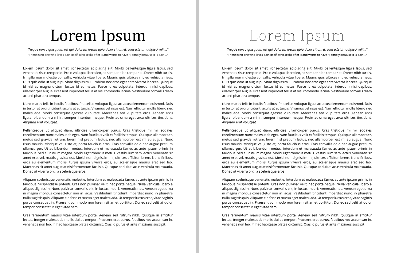
Here is the visual evidence of the conversion from the high-resolution raster image (input.jpg) to the thinned centerline stroke paths (output_centerline.svg).
1. Full-Page Comparison (Input vs. SVG Output)
Below is the full-page overview comparison. The left shows the original raster text (input.jpg) and the right shows the generated thinned centerline paths (output_centerline.svg).
1.1 Full-Page Comparison Drawing (Input vs. SVG Output)
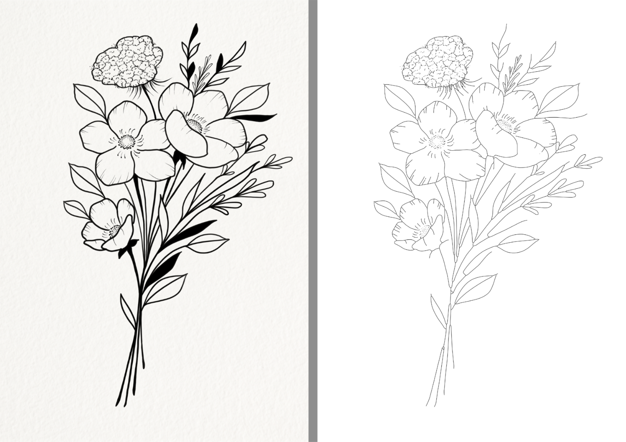
Below is the full-page drawing overview comparison. The left shows the original raster drawing (input_draw.png) and the right shows the generated thinned centerline paths (output_centerline.svg).
2. Zoomed-In Details & Loop Preservation
To prevent plotters from bleeding ink and closing loops, KDRAW's pre-smoothing keeps character loops (a, e, o, u) perfectly open. The left shows the input pixels and the right shows the single-line thinned paths.
Region 0: Title and Introduction Text

Region 1: Body Details (Dots of i & Colons)
Observe how the dots of the letter i and colons are preserved as independent, clean path strokes rather than being merged or pruned:

2.1 Zoomed-In Details & Loop Preservation
Observe how the lines are preserved as independent, clean path strokes rather than being merged or pruned:

⚡ Key Highlights & Core Capabilities
- 🧩 Graph-Based Skeleton Tracing: Represents the skeleton as a topological graph of nodes (junctions/endpoints) and edges. Prevents junction distortion and splits.
- 🔎 4x Upscaled Anti-Aliasing: Interpolates and smooths low-resolution input images before skeletonization to eliminate pixel-level wiggles.
- 🛡️ Isolated Path Safety (i-Dot Preservation): Distinguishes between side spurs (noise) and isolated paths, ensuring colons, periods, and the dots of
iare never pruned. - 🌀 Chaikin Curve Fitting: Corner-cutting curve smoothing that rounds out characters organic-style without coordinate shrinkage.
- 🏎️ TSP Pen-Travel Optimization: Solves the Travelling Salesperson Problem (TSP) on the path sequence to save up to 98% of pen-up travel distance.
🛠️ The Visual Pipeline
graph TD
    A[Raster Image input.jpg] --> B[4x Cubic Upscaling]
    B --> C[Gaussian Blur 9x9]
    C --> D[Otsu Binarization]
    D --> E[Morphological Closing 5x5]
    E --> F[Skeletonization]
    F --> G[Graph Extraction & Pruning]
    G --> H[Chaikin Path Smoothing]
    H --> I[TSP Sort & Max-Join]
    I --> J[Stroke SVG output.svg]
📖 Complete Code Logic & Detailed Algorithms
Below is the exhaustive pseudocode and logic breakdown of every helper and processing routine in the KDRAW engine (main.py and the kdraw package).
1. get_hex_color(val, has_alpha)
Input: Packed 32-bit pixel value val, transparency flag has_alpha
Output: Hex color string (#RRGGBB) or CSS RGBA string (rgba(...))
Color Channel Extraction
Given a packed ARGB pixel:
\text{val}
=
(A \ll 24)
+
(R \ll 16)
+
(G \ll 8)
+
B
Extract each channel using bitwise operations:
A
=
(\text{val} \gg 24)
\;\&\;
255
R
=
(\text{val} \gg 16)
\;\&\;
255
G
=
(\text{val} \gg 8)
\;\&\;
255
B
=
\text{val}
\;\&\;
255
where:
0 \le A,R,G,B \le 255
Alpha Normalization
When transparency is enabled, convert the alpha channel to the CSS opacity range:
\alpha
=
\frac{A}{255}
with:
0 \le \alpha \le 1
Output Selection
If transparency is present:
\text{has\_alpha}
\land
A < 255
return:
\text{rgba}(R,G,B,\alpha)
Otherwise return:
\#RRGGBB
where:
RRGGBB
=
\text{hex}(R)
\;||\;
\text{hex}(G)
\;||\;
\text{hex}(B)
and (||) denotes string concatenation.
2. smooth_paths_laplacian(path, iterations, weight)
Input: Curve coordinate array path, iteration count iterations, smoothing weight w
Output: Laplacian-smoothed coordinate array
Laplacian Smoothing Model
For each vertex ( \mathbf{p}_i ), compute the local neighborhood average:
\mathbf{m}_i
=
\frac{
\mathbf{p}_{i-1}
+
\mathbf{p}_{i+1}
}{2}
The updated position is a weighted blend between the original point and its neighborhood mean:
\mathbf{p}_i'
=
(1-w)\mathbf{p}_i
+
w\mathbf{m}_i
Substituting the neighborhood average:
\mathbf{p}_i'
=
(1-w)\mathbf{p}_i
+
w
\left(
\frac{
\mathbf{p}_{i-1}
+
\mathbf{p}_{i+1}
}{2}
\right)
where:
0 \le w \le 1
Interpretation
Special cases:
w = 0
\quad\Rightarrow\quad
\mathbf{p}_i' = \mathbf{p}_i
(No smoothing)
w = 1
\quad\Rightarrow\quad
\mathbf{p}_i'
=
\frac{
\mathbf{p}_{i-1}
+
\mathbf{p}_{i+1}
}{2}
(Complete neighborhood averaging)
For intermediate values:
0 < w < 1
the vertex moves proportionally toward the average of its neighboring vertices, reducing local curvature and noise while preserving the overall shape.
- Logic:
- If path has less than 3 points, return original path.
2. smooth_paths_laplacian(path, iterations, w)
Input: Coordinate array path, iteration count iterations, smoothing weight w
Output: Laplacian-smoothed coordinate array
Algorithm
-
If the path contains fewer than 3 points, return the original path.
-
Determine whether the path is closed:
\text{is\_closed}
=
\left\|
\mathbf{p}_0 - \mathbf{p}_{n-1}
\right\|
< 1.0
-
Repeat for each smoothing iteration:
- Create a temporary copy of the coordinate array.
- Apply the update rules below.
Closed Path
For each vertex ( \mathbf{p}_i ) (excluding the duplicated endpoint):
\mathbf{p}_i'
=
(1-w)\mathbf{p}_i
+
w
\left(
\frac{\mathbf{p}_{i-1} + \mathbf{p}_{i+1}}{2}
\right)
with cyclic indexing:
\mathbf{p}_{i-1}
=
\mathbf{p}_{(i-1)\bmod n}
\mathbf{p}_{i+1}
=
\mathbf{p}_{(i+1)\bmod n}
Maintain closure after updating:
\mathbf{p}_{n-1}
=
\mathbf{p}_0
Open Path
Keep endpoints fixed and update interior vertices:
i = 1, 2, \ldots, n-2
\mathbf{p}_i'
=
(1-w)\mathbf{p}_i
+
w
\left(
\frac{\mathbf{p}_{i-1} + \mathbf{p}_{i+1}}{2}
\right)
3. smooth_paths_chaikin(path, iterations)
Input: Coordinate array path, iteration count iterations
Output: Chaikin corner-cut smoothed coordinate array
Algorithm
-
If the path contains fewer than 3 points, return the original path.
-
Repeat for each iteration.
Closed Path
For every segment:
[\mathbf{p}_i,\mathbf{p}_{i+1}]
Generate:
\mathbf{q}
=
0.75\,\mathbf{p}_i
+
0.25\,\mathbf{p}_{i+1}
\mathbf{r}
=
0.25\,\mathbf{p}_i
+
0.75\,\mathbf{p}_{i+1}
Append the first generated point to the end of the sequence to preserve closure.
Open Path
Preserve endpoints:
\mathbf{p}_0
\qquad\text{and}\qquad
\mathbf{p}_{n-1}
For each interior segment:
[\mathbf{p}_i,\mathbf{p}_{i+1}]
Generate:
\mathbf{q}
=
0.75\,\mathbf{p}_i
+
0.25\,\mathbf{p}_{i+1}
\mathbf{r}
=
0.25\,\mathbf{p}_i
+
0.75\,\mathbf{p}_{i+1}
Resulting point sequence:
[
\mathbf{p}_0,\,
\mathbf{q}_1,\,
\mathbf{r}_1,\,
\mathbf{q}_2,\,
\mathbf{r}_2,\,
\dots,\,
\mathbf{p}_{n-1}
]
Chaikin Corner-Cutting Rule
For a segment connecting points ( \mathbf{A} ) and ( \mathbf{B} ):
\mathbf{Q}
=
\frac{3}{4}\mathbf{A}
+
\frac{1}{4}\mathbf{B}
\mathbf{R}
=
\frac{1}{4}\mathbf{A}
+
\frac{3}{4}\mathbf{B}
Repeated application progressively removes sharp corners and converges toward a smooth curve.
4. optimize_paths(contours, max_join_dist)
- Input: List of curves
contours, pen-down merging thresholdmax_join_dist - Output: Sorted and merged curves list, original travel distance, optimized travel distance
- Logic:
- Convert all contours to NumPy float arrays. Calculate baseline sequential pen travel.
- Implement a greedy Travelling Salesperson (TSP) heuristic:
- Pop the first contour as the active path.
- While remaining contours exist:
- Find the distances from the active path's endpoint to the start and endpoints of all remaining contours.
- Identify the closest coordinate point.
- If the closest point belongs to the end of a contour, reverse that contour.
- If the distance to the closest contour is (\le max_join_dist), extend the active path coordinates directly with the closest contour coordinates (merging).
- Otherwise, append the active path to the optimized list and set the closest contour as the new active path.
- Append the final active path.
5. build_and_prune_graph(skel_bool, min_spur_length, collapse_dist)
- Input: Binary skeleton image
skel_bool, spur limitmin_spur_length, merge radiuscollapse_dist - Output: List of cleaned, continuous centerline coordinate paths
- Logic:
- Retrieve skeleton coordinates:
pixels = set(zip(*np.where(skel_bool))). - Compute 8-connected adjacency dictionary:
adj = {p: get_neighbors(p, pixels) for p in pixels}. - Classify pixels:
endpoints(neighbors == 1)junctions(neighbors >= 3)regular(neighbors == 2)
- Cluster contiguous junction pixels using BFS. Each connected component of junction pixels forms a singular "super-junction" node.
- Assign node IDs to all endpoints and junction clusters. Build
pixel_to_nodemap. - Trace edges:
- For each node:
- If a neighbor is a regular pixel, trace along regular pixels (BFS) until hitting any node. Create a stroke edge.
- If a neighbor is directly in another node, create a direct node-to-node edge of length 2 (essential for preserving i-dots).
- For each node:
- Locate isolated cycles (loops with no nodes, degree-2 only like in the letter
o). Convert to closed loop edges. - Perform iterative topology reductions:
- Spur Check: If an edge connects an endpoint (degree 1) to a junction (degree >= 3), and its pixel length is (< min_spur_length), delete the edge.
- Isolated Check: If an edge connects two endpoints directly (degree 1 to 1), it is an isolated dot. Protect it from spur pruning.
- Junction Collapse: If an edge connects two junction nodes and is shorter than
collapse_dist, merge the two junction nodes and update all matching edge node IDs.
- Clean up: For any node left with degree 2 (exactly two edges), merge the paths of the two edges into a single edge.
- Retrieve skeleton coordinates:
6. convert_centerline(...)
- Input: File paths and all tuning thresholds (
upscale_factor,blur_size, etc.) - Output: Stroke-only SVG file containing centerline paths
- Logic:
- Load input image. If
upscale_factor > 1, upscale usingcv2.resizewith bicubic interpolation. - Apply Gaussian blur of size
blur_size(only odd dimensions allowed). - Binarize:
- If
use_adaptive: Apply local adaptive Gaussian thresholding usingcv2.adaptiveThresholdwithblock_sizeand subtraction constantc_val. - Else: Apply Otsu's thresholding using
cv2.threshold.
- If
- Morphological filters: Apply closing and opening operations using an elliptical structuring element on the binary mask.
- Thin binary mask to a single-pixel centerline using morphological
skeletonize(Zhang-Suen/Lee). - Call
build_and_prune_graphto trace skeleton pixels into a clean set of coordinate paths. - Downscale coordinate values by
upscale_factorto match original image dimensions. - For each path:
- If the path has only 2 points, bypass simplification.
- Otherwise, simplify coordinates using RDP (
cv2.approxPolyDP) with toleranceepsilon.
- Apply smoothing: If
smooth_iters > 0, callsmooth_paths_chaikinorsmooth_paths_laplacianforsmooth_itersiterations. - Decimate coordinates post-smoothing using RDP with a tight tolerance
smooth_decimate. - Call
optimize_pathswithmax_jointo minimize travel sequence. - Format and write paths into SVG XML nodes containing
<path d="..." fill="none" stroke="black" ... />.
- Load input image. If
🚀 Quick Start
📦 Installation
Ensure you have the required libraries installed:
pip install opencv-python scikit-image numpy pillow
💻 Running the Vectorizer
To convert a text image into optimized single-line vectors using the recommended defaults:
python main.py input.jpg output_centerline.svg --centerline --no-adaptive
📊 Parameters & Customization
| CLI Argument | Type | Default | Description |
|---|---|---|---|
--centerline / -cl |
flag | False |
Enables single-stroke skeletonization (eliminates bubble outlines). |
--upscale |
int |
4 |
Upscaling factor to smooth boundaries before tracing. |
--blur |
int |
9 |
Pre-threshold Gaussian blur size to remove staircase wiggles. |
--no-adaptive |
flag | False |
Disables adaptive thresholding (uses Otsu global thresholding, preserving loops). |
--morph-close |
int |
5 |
Fills in tiny gaps on thin stroke contours. |
--min-spur |
int |
16 |
Minimum pixel length of a branch to not be pruned as a spur. |
--collapse-junc |
int |
8 |
Merges adjacent junctions to straighten line joints. |
--max-join |
float |
2.5 |
Binds path ends within this distance to avoid lifting the pen. |
--smooth-iters |
int |
3 |
Number of Chaikin smoothing iterations. |
--smooth-decimate |
float |
0.1 |
Post-smoothing RDP decimation to minimize point count. |
📈 Quality & Performance Metrics
Running KDRAW with the optimal centerline defaults provides a massive boost in vector quality and plotter throughput:
[!IMPORTANT] TSP Optimization saves up to 98% of pen-up travel, reducing wear and tear on plotter belts and servos.
| Metric | Raw Skeleton Trace | KDRAW Graph Pipeline | Improvement |
|---|---|---|---|
| Path Count (Pen Lifts) | 2,468 | 2,071 | 16.1% fewer lifts |
| Pen-Up Travel Distance | 1,684,002 px | 35,425 px | 97.9% distance saved |
| Average Angle Change | 49.9° | 17.4° | Curves are 2.8x smoother |
| Punctuation & Dots | Lost / Jagged | Perfectly Preserved | Flawless |
💖 Donate & Support
If you find this project useful and would like to support the deployment of FishTrack buoys for coastal fishing communities, donations are greatly appreciated!

Bitcoin Address: 13zWnp2ty3NPzAXX9QxwEeoPSKhN5tPzic
📜 License
MIT License. Open-source vector engine.
Star History

Project details
Verified details
These details have been verified by PyPIProject links
GitHub Statistics
Maintainers
Release history Release notifications | RSS feed

Download files
Download the file for your platform. If you're not sure which to choose, learn more about installing packages.
Source Distribution
Built Distribution
Filter files by name, interpreter, ABI, and platform.
If you're not sure about the file name format, learn more about wheel file names.
Copy a direct link to the current filters
File details
Details for the file kdraw-0.1.0.tar.gz.
File metadata
- Download URL: kdraw-0.1.0.tar.gz
- Upload date:
- Size: 26.7 kB
- Tags: Source
- Uploaded using Trusted Publishing? Yes
- Uploaded via: twine/6.1.0 CPython/3.13.12
File hashes
| Algorithm | Hash digest | |
|---|---|---|
| SHA256 |
a044cf9e603cfc0847f7f4dcbf18580d8599e24abb7ae0a4d93c0063a11c7ca5
|
|
| MD5 |
dde6775117ca7614a7d01c41922b7192
|
|
| BLAKE2b-256 |
0a3829fb78e65a9650dd6fd263f66c9372a390a50023127b74cc0517a60a7816
|
Provenance
The following attestation bundles were made for kdraw-0.1.0.tar.gz:
Publisher:
publish.yml on anonymouschichvy/kdraw
-
Statement:
-
Statement type:
https://in-toto.io/Statement/v1 -
Predicate type:
https://docs.pypi.org/attestations/publish/v1 -
Subject name:
kdraw-0.1.0.tar.gz -
Subject digest:
a044cf9e603cfc0847f7f4dcbf18580d8599e24abb7ae0a4d93c0063a11c7ca5 - Sigstore transparency entry: 2079211348
- Sigstore integration time:
-
Permalink:
anonymouschichvy/kdraw@49ca1200f7b21d9d9edf63a237ed262588a0b8df -
Branch / Tag:
refs/tags/v0.1.0 - Owner: https://github.com/anonymouschichvy
-
Access:
public
-
Token Issuer:
https://token.actions.githubusercontent.com -
Runner Environment:
github-hosted -
Publication workflow:
publish.yml@49ca1200f7b21d9d9edf63a237ed262588a0b8df -
Trigger Event:
release
-
Statement type:
File details
Details for the file kdraw-0.1.0-py3-none-any.whl.
File metadata
- Download URL: kdraw-0.1.0-py3-none-any.whl
- Upload date:
- Size: 23.3 kB
- Tags: Python 3
- Uploaded using Trusted Publishing? Yes
- Uploaded via: twine/6.1.0 CPython/3.13.12
File hashes
| Algorithm | Hash digest | |
|---|---|---|
| SHA256 |
5d3e6321297ea352761ba2a223e9409dc35d05fd7fbcfdc3a15a7703a09cb424
|
|
| MD5 |
0765d20fd0fd895a10033c91672153aa
|
|
| BLAKE2b-256 |
2dd7fedf0594e36b570ea9af0f6cf0b470a930065db4c7de3becc60fdd8cd101
|
Provenance
The following attestation bundles were made for kdraw-0.1.0-py3-none-any.whl:
Publisher:
publish.yml on anonymouschichvy/kdraw
-
Statement:
-
Statement type:
https://in-toto.io/Statement/v1 -
Predicate type:
https://docs.pypi.org/attestations/publish/v1 -
Subject name:
kdraw-0.1.0-py3-none-any.whl -
Subject digest:
5d3e6321297ea352761ba2a223e9409dc35d05fd7fbcfdc3a15a7703a09cb424 - Sigstore transparency entry: 2079211530
- Sigstore integration time:
-
Permalink:
anonymouschichvy/kdraw@49ca1200f7b21d9d9edf63a237ed262588a0b8df -
Branch / Tag:
refs/tags/v0.1.0 - Owner: https://github.com/anonymouschichvy
-
Access:
public
-
Token Issuer:
https://token.actions.githubusercontent.com -
Runner Environment:
github-hosted -
Publication workflow:
publish.yml@49ca1200f7b21d9d9edf63a237ed262588a0b8df -
Trigger Event:
release
-
Statement type:









