

Kimimaro: Skeletonize Densely Labeled Images
# Produce SWC files from volumetric images.
kimimaro forge labels.npy --progress # writes to ./kimimaro_out/
kimimaro view kimimaro_out/10.swc
Rapidly skeletonize all non-zero labels in 2D and 3D numpy arrays using a TEASAR derived method. The returned list of skeletons is in the format used by cloud-volume. A skeleton is a stick figure 1D representation of a 2D or 3D object that consists of a graph of verticies linked by edges. A skeleton where the verticies also carry a distance to the nearest boundary they were extracted from is called a "Medial Axis Transform", which Kimimaro provides.
Skeletons are a compact representation that can be used to visualize objects, trace the connectivity of an object, or otherwise analyze the object's geometry. Kimimaro was designed for use with high resolution neurons extracted from electron microscopy data via AI segmentation, but it can be applied to many different fields.
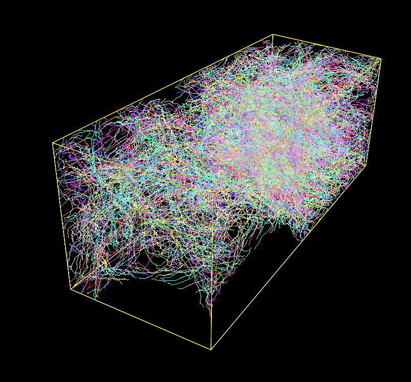
On an Apple Silicon M1 arm64 chip (Firestorm cores 3.2 GHz max frequency), this package processed a 512x512x100 volume with 333 labels in 20 seconds. It processed a 512x512x512 volume (connectomics.npy) with 2124 labels in 187 seconds.
Fig. 1: A Densely Labeled Volume Skeletonized with Kimimaro
pip Installation
If a binary is available for your platform:
pip install kimimaro
# installs additional libraries to accelerate some
# operations like join_close_components
pip install "kimimaro[accel]"
# Makes the kimimaro view command work
pip install "kimimaro[view]"
# Enables TIFF generation on the CLI
pip install "kimimaro[tif]"
# Enables reading NIBABEL, NRRD, TIFF, CRACKLE on the CLI
pip install "kimimaro[all_formats]"
# Install all optional dependencies
pip install "kimimaro[all]"
Otherwise, you'll also need a C++ compiler:
sudo apt-get install python3-dev g++ # ubuntu linux
Example
Fig. 2: Memory Usage on a 512x512x512 Densely Labeled Volume (`connectomics.npy`)
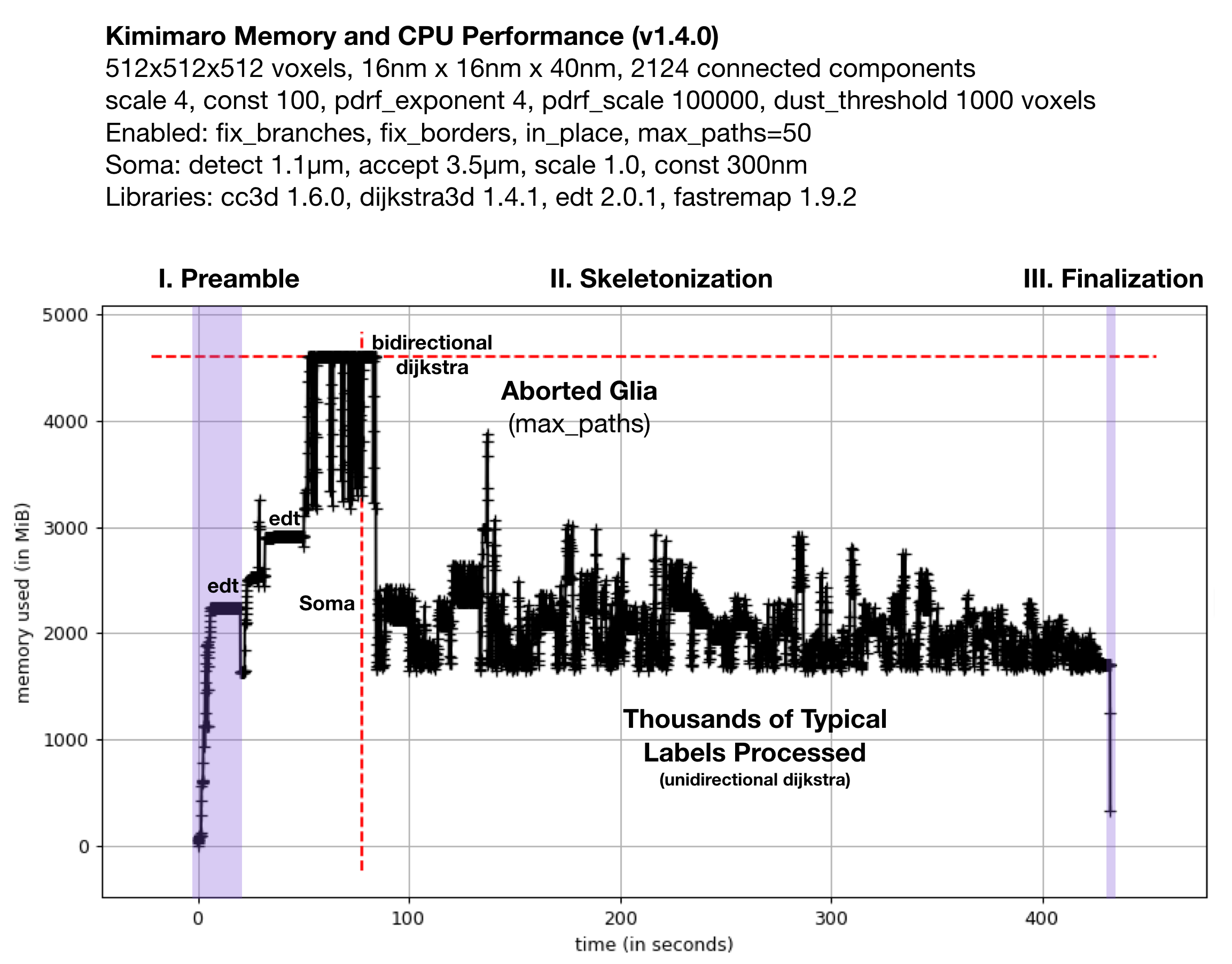
Figure 2 shows the memory usage and processessing time (~390 seconds, about 6.5 minutes) required when Kimimaro 1.4.0 was applied to a 512x512x512 cutout, labels, from a connectomics dataset, connectomics.npy containing 2124 connected components. The different sections of the algorithm are depicted. Grossly, the preamble runs for about half a minute, skeletonization for about six minutes, and finalization within seconds. The peak memory usage was about 4.5 GB. The code below was used to process labels. The processing of the glia was truncated in due to a combination of fix_borders and max_paths.
Kimimaro has come a long way. Version 0.2.1 took over 15 minutes and had a Preamble run time twice as long on the same dataset.
On a Macbook Pro M3, the same settings now complete in 94 seconds (1.6 minutes) on version 5.4.0. With xs3d 1.11.0, cross section analysis takes 215 seconds (3.6 minutes).
Python Interface
# LISTING 1: Producing Skeletons from a labeled image.

import kimimaro

# To obtain this 512 MB segmentation sample volume:
# pip install crackle-codec

import crackle
labels = crackle.load("benchmarks/connectomics.npy.ckl.gz")

skels = kimimaro.skeletonize(
  labels,
  teasar_params={
    "scale": 1.5,
    "const": 300, # physical units
    "pdrf_scale": 100000,
    "pdrf_exponent": 4,
    "soma_acceptance_threshold": 3500, # physical units
    "soma_detection_threshold": 750, # physical units
    "soma_invalidation_const": 300, # physical units
    "soma_invalidation_scale": 2,
    "max_paths": 300, # default None
  },
  # object_ids=[ ... ], # process only the specified labels
  # extra_targets_before=[ (27,33,100), (44,45,46) ], # target points in voxels
  # extra_targets_after=[ (27,33,100), (44,45,46) ], # target points in voxels
  dust_threshold=1000, # skip connected components with fewer than this many voxels
  anisotropy=(16,16,40), # default True
  fix_branching=True, # default True
  fix_borders=True, # default True
  fill_holes=False, # default False
  fix_avocados=False, # default False
  progress=True, # default False, show progress bar
  parallel=1, # <= 0 all cpu, 1 single process, 2+ multiprocess
  parallel_chunk_size=100, # how many skeletons to process before updating progress bar
)

# LISTING 2: Combining skeletons produced from
#            adjacent or overlapping images.

import kimimaro
from osteoid import Skeleton

skels = ... # a set of skeletons produced from the same label id
skel = Skeleton.simple_merge(skels).consolidate()
skel = kimimaro.postprocess(
  skel,
  dust_threshold=1000, # physical units
  tick_threshold=3500 # physical units
)

# LISTING 3: Adding cross sectional area to skeletons
# Cross section planes are defined by normal vectors. Those
# vectors come from the difference between adjacent vertices.
skels = ... # one or more skeletons produced from a single image
skels = kimimaro.cross_sectional_area(
  labels, skels,
  anisotropy=(16,16,40),
  smoothing_window=5, # rolling average window of plane normals
  progress=True,
)
skel = skels[0]
skel.cross_sectional_area # array of cross sectional areas
skel.cross_sectional_area_contacts # non-zero contacted the image border

# Split input skeletons into connected components and
# then join the two nearest vertices within `radius` distance
# of each other until there is only a single connected component
# or no pairs of points nearer than `radius` exist.
# Fuse all remaining components into a single skeleton.
skel = kimimaro.join_close_components([skel1, skel2], radius=1500) # 1500 units threshold
skel = kimimaro.join_close_components([skel1, skel2], radius=None) # no threshold

# Given synapse centroids (in voxels) and the SWC integer label you'd
# like to assign (e.g. for pre-synaptic and post-synaptic) this finds the
# nearest voxel to the centroid for that label.
# Input: { label: [ ((x,y,z), swc_label), ... ] }
# Returns: { (x,y,z): swc_label, ... }
extra_targets = kimimaro.synapses_to_targets(labels, synapses)


# LISTING 4: Drawing a centerline between
#   preselected points on a binary image.
#   This is a much simpler option for when
#   you know exactly what you want, but may
#   be less efficient for large scale procesing.

skel = kimimaro.connect_points(
  labels == 67301298,
  start=(3, 215, 202),
  end=(121, 426, 227),
  anisotropy=(32,32,40),
)

# LISTING 5: Using skeletons to oversegment existing
#  segmentations for integration into proofreading systems
#  that on merging atomic labels. oversegmented_labels
#  is returned numbered from 1. skels is a copy returned
#  with the property skel.segments that associates a label
#  to each vertex (labels will not be unique if downsampling
#  is used)
oversegmented_labels, skels = kimimaro.oversegment(
  labels, skels,
  anisotropy=(32,32,40),
  downsample=10,
)
connectomics.npy is multilabel connectomics data derived from pinky40, a 2018 experimental automated segmentation of ~1.5 million cubic micrometers of mouse visual cortex. It is an early predecessor to the now public pinky100_v185 segmentation that can be found at https://microns-explorer.org/phase1 You will need to run lzma -d connectomics.npy.lzma to obtain the 512x512x512 uint32 volume at 32x32x40 nm3 resolution.
CLI Interface
The CLI supports producing skeletons from a single image as SWCs and viewing the resulting SWC files one at a time. By default, the SWC files are written to ./kimimaro_out/$LABEL.swc.
Here's an equivalent example to the code above.
kimimaro forge labels.npy --scale 4 --const 10 --soma-detect 1100 --soma-accept 3500 --soma-scale 1 --soma-const 300 --anisotropy 16,16,40 --fix-borders --progress
Visualize the your data:
kimimaro view 1241241.swc # visualize skeleton
kimimaro view labels.npy # visualize segmentation
It can also convert binary image skeletons produced by thinning algorithms into SWC files and back. This can be helpful for comparing different skeletonization algorithms or even just using their results.
kimimaro swc from binary_image.tiff # -> binary_image.swc
kimimaro swc to --format tiff binary_image.swc # -> binary_image.tiff or npy
Tweaking kimimaro.skeletonize Parameters
This algorithm works by finding a root point on a 3D object and then serially tracing paths via dijksta's shortest path algorithm through a penalty field to the most distant unvisited point. After each pass, there is a sphere (really a circumscribing cube) that expands around each vertex in the current path that marks part of the object as visited.
For a visual tutorial on the basics of the skeletonization procedure, check out this wiki article: A Pictorial Guide to TEASAR Skeletonization
For more detailed information, read below or the TEASAR paper (though we deviate from TEASAR in a few places). [1]
scale and const
Usually, the most important parameters to tweak are scale and const which control the radius of this invalidation sphere according to the equation r(x,y,z) = scale * DBF(x,y,z) + const where the dimensions are physical (e.g. nanometers, i.e. corrected for anisotropy). DBF(x,y,z) is the physical distance from the shape boundary at that point.
Check out this wiki article to help refine your intuition.
anisotropy
Represents the physical dimension of each voxel. For example, a connectomics dataset might be scanned with an electron microscope at 4nm x 4nm per pixel and stacked in slices 40nm thick. i.e. anisotropy=(4,4,40). You can use any units so long as you are consistent.
dust_threshold
This threshold culls connected components that are smaller than this many voxels.
extra_targets_after and extra_targets_before
extra_targets_after provides additional voxel targets to trace to after the morphological tracing algorithm completes. For example, you might add known synapse locations to the skeleton.
extra_targets_before is the same as extra_targets_after except that the additional targets are front-loaded and the paths that they cover are invalidated. This may affect the results of subsequent morphological tracing.
max_paths
Limits the number of paths that can be drawn for the given label. Certain cells, such as glia, that may not be important for the current analysis may be expensive to process and can be aborted early.
pdrf_scale and pdrf_exponent
The pdrf_scale and pdrf_exponent represent parameters to the penalty equation that takes the euclidean distance field (D) and augments it so that cutting closer to the border is very penalized to make dijkstra take paths that are more centered.
Pr = pdrf_scale * (1 - D / max(D)) pdrf_exponent + (directional gradient < 1.0).
The default settings should work fairly well, but under large anisotropies or with cavernous morphologies, it's possible that you might need to tweak it. If you see the skeleton go haywire inside a large area, it could be a collapse of floating point precision.
soma_acceptance_threshold and soma_detection_threshold
We process somas specially because they do not have a tubular geometry and instead should be represented in a hub and spoke manner. soma_acceptance_threshold is the physical radius (e.g. in nanometers) beyond which we classify a connected component of the image as containing a soma. The distance transform's output is depressed by holes in the label, which are frequently produced by segmentation algorithms on somata. We can fill them, but the hole filling algorithm we use is slow so we would like to only apply it occasionally. Therefore, we set a lower threshold, the soma_acceptance_threshold, beyond which we fill the holes and retest the soma.
soma_invalidation_scale and soma_invalidation_const
Once we have classified a region as a soma, we fix root of the skeletonization algorithm at one of the points of maximum distance from the boundary (usually there is only one). We then mark as visited all voxels around that point in a spherical radius described by r(x,y,z) = soma_invalidation_scale * DBF(x,y,z) + soma_invalidation_const where DBF(x,y,z) is the physical distance from the shape boundary at that point. If done correctly, this can prevent skeletons from being drawn to the boundaries of the soma, and instead pulls the skeletons mainly into the processes extending from the cell body.
fix_borders
This feature makes it easier to connect the skeletons of adjacent image volumes that do not fit in RAM. If enabled, skeletons will be deterministically drawn to the approximate center of the 2D contact area of each place where the shape contacts the border. This can affect the performance of the operation positively or negatively depending on the shape and number of contacts.
fix_branching
You'll probably never want to disable this, but base TEASAR is infamous for forking the skeleton at branch points way too early. This option makes it preferential to fork at a more reasonable place at a significant performance penalty.
fill_holes
Warning: This will remove input labels that are deemed to be holes.
If your segmentation contains artifacts that cause holes to appear in labels, you can preprocess the entire image to eliminate background holes and holes caused by entirely contained inclusions. This option adds a moderate amount of additional processing time at the beginning (perhaps ~30%).
fix_avocados
Avocados are segmentations of cell somata that classify the nucleus separately from the cytoplasm. This is a common problem in automatic segmentations due to the visual similarity of a cell membrane and a nuclear membrane combined with insufficient context.
Skeletonizing an avocado results in a poor skeletonization of the cell soma that will disconnect the nucleus and usually results in too many paths traced around the nucleus. Setting fix_avocados=True attempts to detect and fix these problems. Currently we handle non-avocados, avocados, cells with inclusions, and nested avocados. You can see examples here.
progress
Show a progress bar once the skeletonization phase begins.
parallel
Use a pool of processors to skeletonize faster. Each process allocatable task is the skeletonization of one connected component (so it won't help with a single label that takes a long time to skeletonize). This option also affects the speed of the initial euclidean distance transform, which is parallel enabled and is the most expensive part of the Preamble (described below).
parallel_chunk_size
This only applies when using parallel. This sets the number of skeletons a subprocess will extract before returning control to the main thread, updating the progress bar, and acquiring a new task. If this value is set too low (e.g. < 10-20) the cost of interprocess communication can become significant and even dominant. If it is set too high, task starvation may occur for the other subprocesses if a subprocess gets a particularly hard skeleton and they complete quickly. Progress bar updates will be infrequent if the value is too high as well.
The actual chunk size used will be min(parallel_chunk_size, len(cc_labels) // parallel). cc_labels represents the number of connected components in the sample.
Performance Tips
- If you only need a few labels skeletonized, pass in
object_idsto bypass processing all the others. Ifobject_idscontains only a single label, the masking operation will run faster. - Larger TEASAR parameters scale and const require processing larger invalidation regions per path.
- Set
pdrf_exponentto a small power of two (e.g. 1, 2, 4, 8, 16) for a small speedup. - If you are willing to sacrifice the improved branching behavior, you can set
fix_branching=Falsefor a moderate 1.1x to 1.5x speedup (assuming your TEASAR parameters and data allow branching). - If your dataset contains important cells (that may in fact be the seat of consciousness) but they take significant processing power to analyze, you can save them to savor for later by setting
max_pathsto some reasonable level which will abort and proceed to the next label after the algorithm detects that that at least that many paths will be needed. - Parallel distributes work across connected components and is generally a good idea if you have the cores and memory. Not only does it make single runs proceed faster, but you can also practically use a much larger context; that improves soma processing as they are less likely to be cut off. The Preamble of the algorithm (detailed below) is still single threaded at the moment, so task latency increases with size.
- If
parallel_chunk_sizeis set very low (e.g. < 10) during parallel operation, interprocess communication can become a significant overhead. Try raising this value.
Motivation
The connectomics field commonly generates very large densely labeled volumes of neural tissue. Skeletons are one dimensional representations of two or three dimensional objects. They have many uses, a few of which are visualization of neurons, calculating global topological features, rapidly measuring electrical distances between objects, and imposing tree structures on neurons (useful for computation and user interfaces). There are several ways to compute skeletons and a few ways to define them [4]. After some experimentation, we found that the TEASAR [1] approach gave fairly good results. Other approaches include topological thinning ("onion peeling") and finding the centerline described by maximally inscribed spheres. Ignacio Arganda-Carreras, an alumnus of the Seung Lab, wrote a topological thinning plugin for Fiji called Skeletonize3d.
There are several implementations of TEASAR used in the connectomics field [3][5], however it is commonly understood that implementations of TEASAR are slow and can use tens of gigabytes of memory. Our goal to skeletonize all labels in a petavoxel scale image quickly showed clear that existing sparse implementations are impractical. While adapting a sparse approach to a cloud pipeline, we noticed that there are inefficiencies in repeated evaluation of the Euclidean Distance Transform (EDT), the repeated evaluation of the connected components algorithm, in the construction of the graph used by Dijkstra's algorithm where the edges are implied by the spatial relationships between voxels, in the memory cost, quadratic in the number of voxels, of representing a graph that is implicit in image, in the unnecessarily large data type used to represent relatively small cutouts, and in the repeated downloading of overlapping regions. We also found that the naive implmentation of TEASAR's "rolling invalidation ball" unnecessarily reevaluated large numbers of voxels in a way that could be loosely characterized as quadratic in the skeleton path length.
We further found that commodity implementations of the EDT supported only binary images. We were unable to find any available Python or C++ libraries for performing Dijkstra's shortest path on an image. Commodity implementations of connected components algorithms for images supported only binary images. Therefore, several libraries were devised to remedy these deficits (see Related Projects).
Why TEASAR?
TEASAR: Tree-structure Extraction Algorithm for Accurate and Robust skeletons, a 2000 paper by M. Sato and others [1], is a member of a family of algorithms that transform two and three dimensional structures into a one dimensional "skeleton" embedded in that higher dimension. One might concieve of a skeleton as extracting a stick figure drawing from a binary image. This problem is more difficult than it might seem. There are different situations one must consider when making such a drawing. For example, a stick drawing of a banana might merely be a curved centerline and a drawing of a doughnut might be a closed loop. In our case of analyzing neurons, sometimes we want the skeleton to include spines, short protrusions from dendrites that usually have synapses attached, and sometimes we want only the characterize the run length of the main trunk of a neurite.
Additionally, data quality issues can be challenging as well. If one is skeletonizing a 2D image of a doughnut, but the angle were sufficiently declinated from the ring's orthogonal axis, would it even be possible to perform this task accurately? In a 3D case, if there are breaks or mergers in the labeling of a neuron, will the algorithm function sensibly? These issues are common in both manual and automatic image sementations.
In our problem domain of skeletonizing neurons from anisotropic voxel labels, our chosen algorithm should produce tree structures, handle fine or coarse detail extraction depending on the circumstances, handle voxel anisotropy, and be reasonably efficient in CPU and memory usage. TEASAR fufills these criteria. Notably, TEASAR doesn't guarantee the centeredness of the skeleton within the shape, but it makes an effort. The basic TEASAR algorithm is known to cut corners around turns and branch too early. A 2001 paper by members of the original TEASAR team describes a method for reducing the early branching issue on page 204, section 4.2.2. [2]
TEASAR Derived Algorithm
We implemented TEASAR but made several deviations from the published algorithm in order to improve path centeredness, increase performance, handle bulging cell somas, and enable efficient chunked evaluation of large images. We opted not to implement the gradient vector field step from [2] as our implementation is already quite fast. The paper claims a reduction of 70-85% in input voxels, so it might be worth investigating.
In order to work with images that contain many labels, our general strategy is to perform as many actions as possible in such a way that all labels are treated in a single pass. Several of the component algorithms (e.g. connected components, euclidean distance transform) in our implementation can take several seconds per a pass, so it is important that they not be run hundreds or thousands of times. A large part of the engineering contribution of this package lies in the efficiency of these operations which reduce the runtime from the scale of hours to minutes.
Given a 3D labeled voxel array, I, with N >= 0 labels, and ordered triple describing voxel anisotropy A, our algorithm can be divided into three phases, the pramble, skeletonization, and finalization in that order.
I. Preamble
The Preamble takes a 3D image containing N labels and efficiently generates the connected components, distance transform, and bounding boxes needed by the skeletonization phase.
- To enhance performance, if N is 0 return an empty set of skeletons.
- Label the M connected components, Icc, of I.
- To save memory, renumber the connected components in order from 1 to M. Adjust the data type of the new image to the smallest uint type that will contain M and overwrite Icc.
- Generate a mapping of the renumbered Icc to I to assign meaningful labels to skeletons later on and delete I to save memory.
- Compute E, the multi-label anisotropic Euclidean Distance Transform of Icc given A. E treats all interlabel edges as transform edges, but not the boundaries of the image. Black pixels are considered background.
- Gather a list, Lcc of unique labels from Icc and threshold which ones to process based on the number of voxels they represent to remove "dust".
- In one pass, compute the list of bounding boxes, B, corresponding to each label in Lcc.
II. Skeletonization
In this phase, we extract the tree structured skeleton from each connected component label. Below, we reference variables defined in the Preamble. For clarity, we omit the soma specific processing and hold fix_branching=True.
For each label l in Lcc and B...
- Extract Il, the cropped binary image tightly enclosing l from Icc using Bl
- Using Il and Bl, extract El from E. El is the cropped tightly enclosed EDT of l. This is much faster than recomputing the EDT for each binary image.
- Find an arbitrary foreground voxel and using that point as a source, compute the anisotropic euclidean distance field for Il. The coordinate of the maximum value is now "the root" r.
- From r, compute the euclidean distance field and save it as the distance from root field Dr.
- Compute the penalized distance from root field Pr =
pdrf_scale* ((1 - El / max(El)) ^pdrf_exponent) + Dr / max(Dr). - While Il contains foreground voxels:
- Identify a target coordinate, t, as the foreground voxel with maximum distance in Dr from r.
- Draw the shortest path p from r to t considering the voxel values in Pr as edge weights.
- For each vertex v in p, extend an invalidation cube of physical side length computed as
scale* El(v) +constand convert any foreground pixels in Il that overlap with these cubes to background pixels. - (Only if
fix_branching=True) For each vertex coordinate v in p, set Pr(v) = 0. - Append p to a list of paths for this label.
- Using El, extract the distance to the nearest boundary each vertex in the skeleton represents.
- For each raw skeleton extracted from Il, translate the vertices by Bl to correct for the translation the cropping operation induced.
- Multiply the vertices by the anisotropy A to place them in physical space.
If soma processing is considered, we modify the root (r) search process as follows:
- If max(El) >
soma_detection_threshold... - Fill toplogical holes in Il. Soma are large regions that often have dust from imperfect automatic labeling methods.
- Recompute El from this cleaned up image.
- If max(El) >
soma_acceptance_threshold, divert to soma processing mode. - If in soma processing mode, continue, else go to step 3 in the algorithm above.
- Set r to the coordinate corresponding to max(El)
- Create an invalidation sphere of physical radius
soma_invalidation_scale* max(El) +soma_invalidation_constand erase foreground voxels from Il contained within it. This helps prevent errant paths from being drawn all over the soma. - Continue from step 4 in the above algorithm.
III. Finalization
In the final phase, we agglomerate the disparate connected component skeletons into single skeletons and assign their labels corresponding to the input image. This step is artificially broken out compared to how intermingled its implementation is with skeletonization, but it's conceptually separate.
Deviations from TEASAR
There were several places where we took a different approach than called for by the TEASAR authors.
Using DAF for Targets, PDRF for Pathfinding
The original TEASAR algorithm defines the Penalized Distance from Root voxel Field (PDRF, Pr above) as:
PDRF = 5000 * (1 - DBF / max(DBF))^16 + DAF
DBF is the Distance from Boundary Field (El above) and DAF is the Distance from Any voxel Field (Dr above).
We found the addition of the DAF tended to perturb the skeleton path from the centerline better described by the inverted DBF alone. We also found it helpful to modify the constant and exponent to tune cornering behavior. Initially, we completely stripped out the addition of the DAF from the PDRF, but this introduced a different kind of problem. The exponentiation of the PDRF caused floating point values to collapse in wide open spaces. This made the skeletons go crazy as they traced out a path described by floating point errors.
The DAF provides a very helpful gradient to follow between the root and the target voxel, we just don't want that gradient to knock the path off the centerline. Therefore, in light of the fact that the PDRF base field is very large, we add the normalized DAF which is just enough to overwhelm floating point errors and provide direction in wide tubes and bulges.
The original paper also called for selecting targets using the max(PDRF) foreground values. However, this is a bit strange since the PDRF values are dominated by boundary effects rather than a pure distance metric. Therefore, we select targets from the max(DAF) forground value.
Zero Weighting Previous Paths (fix_branching=True)
The 2001 skeletonization paper [2] called for correcting early forking by computing a DAF using already computed path vertices as field sources. This allows Dijkstra's algorithm to trace the existing path cost free and diverge from it at a closer point to the target.
As we have strongly deemphasized the role of the DAF in dijkstra path finding, computing this field is unnecessary and we only need to set the PDRF to zero along the path of existing skeletons to achieve this effect. This saves us an expensive repeated DAF calculation per path.
However, we still incur a substantial cost for taking this approach because we had been computing a dijkstra "parental field" that recorded the shortest path to the root from every foreground voxel. We then used this saved result to rapidly compute all paths. However, as this zero weighting modification makes successive calculations dependent upon previous ones, we need to compute Dijkstra's algorithm anew for each path.
Non-Overlapped Chunked Processing (fix_borders=True)
When processing large volumes, a sensible approach for mass producing skeletons is to chunk the volume, process the chunks independently, and merge the resulting skeleton fragments at the end. However, this is complicated by the "edge effect" induced by a loss of context which makes it impossible to expect the endpoints of skeleton fragments produced by adjacent chunks to align. In contrast, it is easy to join mesh fragments because the vertices of the edge of mesh fragments lie at predictable identical locations given one pixel of overlap.
Previously, we had used 50% overlap to join adjacent skeleton fragments which increased the compute cost of skeletonizing a large volume by eight times. However, if we could force skeletons to lie at predictable locations on the border, we could use single pixel overlap and copy the simple mesh joining approach. As an (incorrect but useful) intuition for how one might go about this, consider computing the centroid of each connected component on each border plane and adding that as a required path target. This would guarantee that both sides of the plane connect at the same pixel. However, the centroid may not lie inside of non-convex hulls so we have to be more sophisticated and select some real point inside of the shape.
To this end, we again repurpose the euclidean distance transform and apply it to each of the six planes of connected components and select the maximum value as a mandatory target. This works well for many types of objects that contact a single plane and have a single maximum. However, we must treat the corners of the box and shapes that have multiple maxima.
To handle shapes that contact multiple sides of the box, we simply assign targets to all connected components. If this introduces a cycle in post-processing, we already have cycle removing code to handle it in Igneous. If it introduces tiny useless appendages, we also have code to handle this.
If a shape has multiple distance transform maxima, it is important to choose the same pixel without needing to communicate between spatially adjacent tasks which may run at different times on different machines. Additionally, the same plane on adjacent tasks has the coordinate system flipped. One simple approach might be to pick the coordinate with minimum x and y (or some other coordinate based criterion) in one of the coordinate frames, but this requires tracking the flips on all six planes and is annoying. Instead, we use a series of coordinate-free topology based filters which is both more fun, effort efficient, and picks something reasonable looking. A valid criticism of this approach is that it will fail on a perfectly symmetrical object, but these objects are rare in biological data.
We apply a series of filters and pick the point based on the first filter it passes:
- The voxel closest to the centroid of the current label.
- The voxel closest to the centroid of the image plane.
- Closest to a corner of the plane.
- Closest to an edge of the plane.
- The previously found maxima.
It is important that filter #1 be based on the shape of the label so that kinks are minimimized for convex hulls. For example, originally we used only filters two thru five, but this caused skeletons for neurites located away from the center of a chunk to suddenly jink towards the center of the chunk at chunk boundaries.
Related Projects
Several classic algorithms had to be specially tuned to make this module possible.
- edt: A single pass, multi-label anisotropy supporting euclidean distance transform implementation.
- dijkstra3d: Dijkstra's shortest-path algorithm defined on 26-connected 3D images. This avoids the time cost of edge generation and wasted memory of a graph representation.
- connected-components-3d: A connected components implementation defined on 26-connected 3D images with multiple labels.
- fastremap: Allows high speed renumbering of labels from 1 in a 3D array in order to reduce memory consumption caused by unnecessarily large 32 and 64-bit labels.
- fill_voids: High speed binary_fill_holes.
- xs3d: Cross section analysis of 3D images.
This module was originally designed to be used with CloudVolume and Igneous.
- CloudVolume: Serverless client for reading and writing petascale chunked images of neural tissue, meshes, and skeletons.
- Igneous: Distributed computation for visualizing connectomics datasets.
Some of the TEASAR modifications used in this package were first demonstrated by Alex Bae.
- skeletonization: Python implementation of modified TEASAR for sparse labels.
Credits
Alex Bae developed the precursor skeletonization package and several modifications to TEASAR that we use in this package. Alex also developed the postprocessing approach used for stitching skeletons using 50% overlap. Will Silversmith adapted these techniques for mass production, refined several basic algorithms for handling thousands of labels at once, and rewrote them into the Kimimaro package. Will added trickle DAF, zero weighted previously explored paths, and fixing borders to the algorithm. A.M. Wilson and Will designed the nucleus/soma "avocado" fuser. Forrest Collman added parameter flexibility and helped tune DAF computation performance. Sven Dorkenwald and Forrest both provided helpful discussions and feedback. Peter Li redesigned the target selection algorithm to avoid bilinear performance on complex cells.
Acknowledgments
We are grateful to our partners in the Seung Lab, the Allen Institute for Brain Science, and the Baylor College of Medicine for providing the data and problems necessitating this library.
This research was supported by the Intelligence Advanced Research Projects Activity (IARPA) via Department of Interior/ Interior Business Center (DoI/IBC) contract number D16PC0005, NIH/NIMH (U01MH114824, U01MH117072, RF1MH117815), NIH/NINDS (U19NS104648, R01NS104926), NIH/NEI (R01EY027036), and ARO (W911NF-12-1-0594). The U.S. Government is authorized to reproduce and distribute reprints for Governmental purposes notwithstanding any copyright annotation thereon. Disclaimer: The views and conclusions contained herein are those of the authors and should not be interpreted as necessarily representing the official policies or endorsements, either expressed or implied, of IARPA, DoI/IBC, or the U.S. Government. We are grateful for assistance from Google, Amazon, and Intel.
Papers Using Kimimaro
Please cite Kimimaro using the CITATION.cff file located in this repository.
The below list is not comprehensive and is sourced from collaborators or found using internet searches and does not constitute an endorsement except to the extent that they used it for their work.
- A.M. Wilson, R. Schalek, A. Suissa-Peleg, T.R. Jones, S. Knowles-Barley, H. Pfister, J.M. Lichtman. "Developmental Rewiring between Cerebellar Climbing Fibers and Purkinje Cells Begins with Positive Feedback Synapse Addition". Cell Reports. Vol. 29, Iss. 9, November 2019. Pgs. 2849-2861.e6 doi: 10.1016/j.celrep.2019.10.081 (link)
- S. Dorkenwald, N.L. Turner, T. Macrina, K. Lee, R. Lu, J. Wu, A.L. Bodor, A.A. Bleckert, D. Brittain, N. Kemnitz, W.M. Silversmith, D. Ih, J. Zung, A. Zlateski, I. Tartavull, S. Yu, S. Popovych, W. Wong, M. Castro, C. S. Jordan, A.M. Wilson, E. Froudarakis, J. Buchanan, M. Takeno, R. Torres, G. Mahalingam, F. Collman, C. Schneider-Mizell, D.J. Bumbarger, Y. Li, L. Becker, S. Suckow, J. Reimer, A.S. Tolias, N. Maçarico da Costa, R. C. Reid, H.S. Seung. "Binary and analog variation of synapses between cortical pyramidal neurons". bioRXiv. December 2019. doi: 10.1101/2019.12.29.890319 (link)
- N.L. Turner, T. Macrina, J.A. Bae, R. Yang, A.M. Wilson, C. Schneider-Mizell, K. Lee, R. Lu, J. Wu, A.L. Bodor, A.A. Bleckert, D. Brittain, E. Froudarakis, S. Dorkenwald, F. Collman, N. Kemnitz, D. Ih, W.M. Silversmith, J. Zung, A. Zlateski, I. Tartavull, S. Yu, S. Popovych, S. Mu, W. Wong, C.S. Jordan, M. Castro, J. Buchanan, D.J. Bumbarger, M. Takeno, R. Torres, G. Mahalingam, L. Elabbady, Y. Li, E. Cobos, P. Zhou, S. Suckow, L. Becker, L. Paninski, F. Polleux, J. Reimer, A.S. Tolias, R.C. Reid, N. Maçarico da Costa, H.S. Seung. "Multiscale and multimodal reconstruction of cortical structure and function". bioRxiv. October 2020; doi: 10.1101/2020.10.14.338681 (link)
- P.H. Li, L.F. Lindsey, M. Januszewski, Z. Zheng, A.S. Bates, I. Taisz, M. Tyka, M. Nichols, F. Li, E. Perlman, J. Maitin-Shepard, T. Blakely, L. Leavitt, G. S.X.E. Jefferis, D. Bock, V. Jain. "Automated Reconstruction of a Serial-Section EM Drosophila Brain with Flood-Filling Networks and Local Realignment". bioRxiv. October 2020. doi: 10.1101/605634 (link)
References
- M. Sato, I. Bitter, M.A. Bender, A.E. Kaufman, and M. Nakajima. "TEASAR: Tree-structure Extraction Algorithm for Accurate and Robust Skeletons". Proc. 8th Pacific Conf. on Computer Graphics and Applications. Oct. 2000. doi: 10.1109/PCCGA.2000.883951 (link)
- I. Bitter, A.E. Kaufman, and M. Sato. "Penalized-distance volumetric skeleton algorithm". IEEE Transactions on Visualization and Computer Graphics Vol. 7, Iss. 3, Jul-Sep 2001. doi: 10.1109/2945.942688 (link)
- T. Zhao, S. Plaza. "Automatic Neuron Type Identification by Neurite Localization in the Drosophila Medulla". Sept. 2014. arXiv:1409.1892 [q-bio.NC] (link)
- A. Tagliasacchi, T. Delame, M. Spagnuolo, N. Amenta, A. Telea. "3D Skeletons: A State-of-the-Art Report". May 2016. Computer Graphics Forum. Vol. 35, Iss. 2. doi: 10.1111/cgf.12865 (link)
- P. Li, L. Lindsey, M. Januszewski, Z. Zheng, A. Bates, I. Taisz, M. Tyka, M. Nichols, F. Li, E. Perlman, J. Maitin-Shepard, T. Blakely, L. Leavitt, G. Jefferis, D. Bock, V. Jain. "Automated Reconstruction of a Serial-Section EM Drosophila Brain with Flood-Filling Networks and Local Realignment". April 2019. bioRXiv. doi: 10.1101/605634 (link)
- M.M. McKerns, L. Strand, T. Sullivan, A. Fang, M.A.G. Aivazis, "Building a framework for predictive science", Proceedings of the 10th Python in Science Conference, 2011; http://arxiv.org/pdf/1202.1056
- Michael McKerns and Michael Aivazis, "pathos: a framework for heterogeneous computing", 2010- ; http://trac.mystic.cacr.caltech.edu/project/pathos
1 maintainer

Metadata
1 maintainer
Release files for kimimaro 5.8.5
For a detailed explanation of source distributions (sdists) and built distributions (wheels), please see the package formats documentation.
Source distribution (sdist)
| File | Size | Uploaded | |
|---|---|---|---|
| kimimaro-5.8.5.tar.gz | 528.3 kB | Details |
Built distributions (wheels)
Total release size: 49.0 MB
Release files / kimimaro-5.8.5.tar.gz
| Download URL | kimimaro-5.8.5.tar.gz |
|---|---|
| Size | 528.3 kB |
| Tags | Source |
|
SHA-256 checksum How to use checksums |
951d62352e0b75cc3667fbc17969a1a14d3f18523976c9fb4a378199ff7bc41a
|
|
BLAKE2b-256 checksum How to use checksums |
6c13bb17e49e823c18cebec80dd35ecd2c47b9a6d099a85996818b72fa5f83c4
|
| Upload date | |
|
Uploaded using Trusted Publishing? What is trusted publishing? |
No |
| Uploaded via |
twine/6.1.0 CPython/3.11.3
|
Release files / kimimaro-5.8.5-cp314-cp314t-win_amd64.whl
| Download URL | kimimaro-5.8.5-cp314-cp314t-win_amd64.whl |
|---|---|
| Size | 333.0 kB |
| Tags | CPython 3.14 CPython 3.14 free-threading Windows x86-64 |
|
SHA-256 checksum How to use checksums |
13fa2d467049990097fd73f5363f20d2fbddd0928ed1ef4c60355c59d8000e63
|
|
BLAKE2b-256 checksum How to use checksums |
67d230cb5779f7c7322f83df15dd8710c01adf23a17fef5c4891593bb20cf5fc
|
| Upload date | |
|
Uploaded using Trusted Publishing? What is trusted publishing? |
No |
| Uploaded via |
twine/6.1.0 CPython/3.11.3
|
Release files / kimimaro-5.8.5-cp314-cp314t-win32.whl
| Download URL | kimimaro-5.8.5-cp314-cp314t-win32.whl |
|---|---|
| Size | 285.4 kB |
| Tags | CPython 3.14 CPython 3.14 free-threading Windows x86-32 |
|
SHA-256 checksum How to use checksums |
417ed2300bced01890b551ec3a51c1d82115d607a3b8f72d899c293576a20d53
|
|
BLAKE2b-256 checksum How to use checksums |
3c701c75f1fb22e964f7981d7fe92cc1402ff07971a46bc24d25e4e5744a78ff
|
| Upload date | |
|
Uploaded using Trusted Publishing? What is trusted publishing? |
No |
| Uploaded via |
twine/6.1.0 CPython/3.11.3
|
Release files / kimimaro-5.8.5-cp314-cp314t-manylinux_2_24_x86_64.manylinux_2_28_x86_64.whl
| Download URL | kimimaro-5.8.5-cp314-cp314t-manylinux_2_24_x86_64.manylinux_2_28_x86_64.whl |
|---|---|
| Size | 2.8 MB |
| Tags | CPython 3.14 CPython 3.14 free-threading Linux glibc 2.24+ x86-64 Linux glibc 2.28+ x86-64 |
|
SHA-256 checksum How to use checksums |
40946799a943a77972be9448ed25c5ca73ac11a1459461f07bec679c10c3ac61
|
|
BLAKE2b-256 checksum How to use checksums |
23af9f3ddcc0c3e0db89340b812f0f763e49a8b31c319f75fa4382f0ea83123a
|
| Upload date | |
|
Uploaded using Trusted Publishing? What is trusted publishing? |
No |
| Uploaded via |
twine/6.1.0 CPython/3.11.3
|
Release files / kimimaro-5.8.5-cp314-cp314t-manylinux_2_24_aarch64.manylinux_2_28_aarch64.whl
| Download URL | kimimaro-5.8.5-cp314-cp314t-manylinux_2_24_aarch64.manylinux_2_28_aarch64.whl |
|---|---|
| Size | 2.8 MB |
| Tags | CPython 3.14 CPython 3.14 free-threading Linux glibc 2.24+ ARM64 Linux glibc 2.28+ ARM64 |
|
SHA-256 checksum How to use checksums |
6bfc5aa62160caec781f21f82538ac95abcba0e686b47ca58d284f0b0fadf65c
|
|
BLAKE2b-256 checksum How to use checksums |
7a411333988fb3da362aba411e3647b06bb70e897d43e98bd7b31663937eab1e
|
| Upload date | |
|
Uploaded using Trusted Publishing? What is trusted publishing? |
No |
| Uploaded via |
twine/6.1.0 CPython/3.11.3
|
Release files / kimimaro-5.8.5-cp314-cp314t-macosx_11_0_arm64.whl
| Download URL | kimimaro-5.8.5-cp314-cp314t-macosx_11_0_arm64.whl |
|---|---|
| Size | 358.2 kB |
| Tags | CPython 3.14 CPython 3.14 free-threading macOS 11.0+ ARM64 |
|
SHA-256 checksum How to use checksums |
8e134cfcaad6e40ee3287517e582f752a239e4c8a5f16152bd3fc5424b25b9b8
|
|
BLAKE2b-256 checksum How to use checksums |
c412280bbcfd1f5508356c5d0f014c9bd48fac070b61ece1df3a590ec8ab2475
|
| Upload date | |
|
Uploaded using Trusted Publishing? What is trusted publishing? |
No |
| Uploaded via |
twine/6.1.0 CPython/3.11.3
|
Release files / kimimaro-5.8.5-cp314-cp314t-macosx_10_13_x86_64.whl
| Download URL | kimimaro-5.8.5-cp314-cp314t-macosx_10_13_x86_64.whl |
|---|---|
| Size | 381.5 kB |
| Tags | CPython 3.14 CPython 3.14 free-threading macOS 10.13+ x86-64 |
|
SHA-256 checksum How to use checksums |
79723b0f69b766763efa7442886fe2d494aaacdc9723e518f96188e5e20f2e58
|
|
BLAKE2b-256 checksum How to use checksums |
f3fcdd7c482e983849a55f808713791a0957f4a6f7d14c75c95df8e5a12d30b9
|
| Upload date | |
|
Uploaded using Trusted Publishing? What is trusted publishing? |
No |
| Uploaded via |
twine/6.1.0 CPython/3.11.3
|
Release files / kimimaro-5.8.5-cp314-cp314-win_amd64.whl
| Download URL | kimimaro-5.8.5-cp314-cp314-win_amd64.whl |
|---|---|
| Size | 310.4 kB |
| Tags | CPython 3.14 Windows x86-64 |
|
SHA-256 checksum How to use checksums |
39b6ec93a03fb4fba81005f60b618ad631a8d111ad2b2683f02f8cc57f265599
|
|
BLAKE2b-256 checksum How to use checksums |
003e4dc80398a9b8ec0742a6a875ef382ca8ec789763f4c7db631f83db8af9ea
|
| Upload date | |
|
Uploaded using Trusted Publishing? What is trusted publishing? |
No |
| Uploaded via |
twine/6.1.0 CPython/3.11.3
|
Release files / kimimaro-5.8.5-cp314-cp314-win32.whl
| Download URL | kimimaro-5.8.5-cp314-cp314-win32.whl |
|---|---|
| Size | 266.7 kB |
| Tags | CPython 3.14 Windows x86-32 |
|
SHA-256 checksum How to use checksums |
0e32d13096737064c1c993207d1bfe211f4a92d2ae48a21e893f3d2514301e01
|
|
BLAKE2b-256 checksum How to use checksums |
f4be76128ccc322f45d865223d23eb47fad701e5fee54a9462c4b1ab09c3d6e7
|
| Upload date | |
|
Uploaded using Trusted Publishing? What is trusted publishing? |
No |
| Uploaded via |
twine/6.1.0 CPython/3.11.3
|
Release files / kimimaro-5.8.5-cp314-cp314-manylinux_2_24_x86_64.manylinux_2_28_x86_64.whl
| Download URL | kimimaro-5.8.5-cp314-cp314-manylinux_2_24_x86_64.manylinux_2_28_x86_64.whl |
|---|---|
| Size | 2.8 MB |
| Tags | CPython 3.14 Linux glibc 2.24+ x86-64 Linux glibc 2.28+ x86-64 |
|
SHA-256 checksum How to use checksums |
6fb4dc8a90152135f34da5301d29693dfff1a3646af66b154f1d6177fc5f5903
|
|
BLAKE2b-256 checksum How to use checksums |
0fb3f41530ffa711c45f0f04d395588b76ed479c0b0321019a4487e751c8a5c0
|
| Upload date | |
|
Uploaded using Trusted Publishing? What is trusted publishing? |
No |
| Uploaded via |
twine/6.1.0 CPython/3.11.3
|
Release files / kimimaro-5.8.5-cp314-cp314-manylinux_2_24_aarch64.manylinux_2_28_aarch64.whl
| Download URL | kimimaro-5.8.5-cp314-cp314-manylinux_2_24_aarch64.manylinux_2_28_aarch64.whl |
|---|---|
| Size | 2.8 MB |
| Tags | CPython 3.14 Linux glibc 2.24+ ARM64 Linux glibc 2.28+ ARM64 |
|
SHA-256 checksum How to use checksums |
a50e791bf8120e4e8c8bd480224b4866a197302278f8f68502ea915425bc9c51
|
|
BLAKE2b-256 checksum How to use checksums |
5e751c2d49cdb623eb20ad25e71cf81b2cbaa7bcc57b08ce10beec0e44c2bc97
|
| Upload date | |
|
Uploaded using Trusted Publishing? What is trusted publishing? |
No |
| Uploaded via |
twine/6.1.0 CPython/3.11.3
|
Release files / kimimaro-5.8.5-cp314-cp314-macosx_11_0_arm64.whl
| Download URL | kimimaro-5.8.5-cp314-cp314-macosx_11_0_arm64.whl |
|---|---|
| Size | 336.4 kB |
| Tags | CPython 3.14 macOS 11.0+ ARM64 |
|
SHA-256 checksum How to use checksums |
372723fe8b5ca607dc76f2539632227e4d9f02050afa56d0b7fdb89b51d5a033
|
|
BLAKE2b-256 checksum How to use checksums |
fb74ddebc184bb2aa7e11436044f4264b08b21820b89c5c88b51b56d76fe6194
|
| Upload date | |
|
Uploaded using Trusted Publishing? What is trusted publishing? |
No |
| Uploaded via |
twine/6.1.0 CPython/3.11.3
|
Release files / kimimaro-5.8.5-cp314-cp314-macosx_10_13_x86_64.whl
| Download URL | kimimaro-5.8.5-cp314-cp314-macosx_10_13_x86_64.whl |
|---|---|
| Size | 361.7 kB |
| Tags | CPython 3.14 macOS 10.13+ x86-64 |
|
SHA-256 checksum How to use checksums |
619abbd3bd9dd5ffd1a5100b8a99fba633ec38de336a426c716ec8a18b1565f1
|
|
BLAKE2b-256 checksum How to use checksums |
7604005cadf90189bd7e918018adbcbf6458b3ef8fa5919539b9891b89db6581
|
| Upload date | |
|
Uploaded using Trusted Publishing? What is trusted publishing? |
No |
| Uploaded via |
twine/6.1.0 CPython/3.11.3
|
Release files / kimimaro-5.8.5-cp313-cp313-win_amd64.whl
| Download URL | kimimaro-5.8.5-cp313-cp313-win_amd64.whl |
|---|---|
| Size | 303.6 kB |
| Tags | CPython 3.13 Windows x86-64 |
|
SHA-256 checksum How to use checksums |
30f3d8557888ff849afc55706f6fd16450d6678f56f8b3364a08d255443b7c38
|
|
BLAKE2b-256 checksum How to use checksums |
0ab035beb6aef864f8a61c7578a3a4da806d90588315863ea69c3f0794d0f48b
|
| Upload date | |
|
Uploaded using Trusted Publishing? What is trusted publishing? |
No |
| Uploaded via |
twine/6.1.0 CPython/3.11.3
|
Release files / kimimaro-5.8.5-cp313-cp313-win32.whl
| Download URL | kimimaro-5.8.5-cp313-cp313-win32.whl |
|---|---|
| Size | 261.1 kB |
| Tags | CPython 3.13 Windows x86-32 |
|
SHA-256 checksum How to use checksums |
32d847b2e542c80b184a7b77604d967e692079204cc8dd3042f665476a6b82b5
|
|
BLAKE2b-256 checksum How to use checksums |
da6a14d098ff8e5a6961bd6809284d576f99a44158d083274a20694be8670952
|
| Upload date | |
|
Uploaded using Trusted Publishing? What is trusted publishing? |
No |
| Uploaded via |
twine/6.1.0 CPython/3.11.3
|
Release files / kimimaro-5.8.5-cp313-cp313-manylinux_2_24_x86_64.manylinux_2_28_x86_64.whl
| Download URL | kimimaro-5.8.5-cp313-cp313-manylinux_2_24_x86_64.manylinux_2_28_x86_64.whl |
|---|---|
| Size | 2.9 MB |
| Tags | CPython 3.13 Linux glibc 2.24+ x86-64 Linux glibc 2.28+ x86-64 |
|
SHA-256 checksum How to use checksums |
46d5d30219886a81873323b189d4ef30ffa45dec79e90456805f3542b71b4ae3
|
|
BLAKE2b-256 checksum How to use checksums |
265935cb63f57ac2aced2a80445bb89f88505c748fe29ccc12f046cb47ad3c10
|
| Upload date | |
|
Uploaded using Trusted Publishing? What is trusted publishing? |
No |
| Uploaded via |
twine/6.1.0 CPython/3.11.3
|
Release files / kimimaro-5.8.5-cp313-cp313-manylinux_2_24_aarch64.manylinux_2_28_aarch64.whl
| Download URL | kimimaro-5.8.5-cp313-cp313-manylinux_2_24_aarch64.manylinux_2_28_aarch64.whl |
|---|---|
| Size | 2.8 MB |
| Tags | CPython 3.13 Linux glibc 2.24+ ARM64 Linux glibc 2.28+ ARM64 |
|
SHA-256 checksum How to use checksums |
fb87c850fa442c54f0a90665e90779df9ef39d215167f5399d68beab0c9e6c1d
|
|
BLAKE2b-256 checksum How to use checksums |
544ae5972e11e028611789dea3bda92a00ea94d82b713d7ee3df0053e36363e9
|
| Upload date | |
|
Uploaded using Trusted Publishing? What is trusted publishing? |
No |
| Uploaded via |
twine/6.1.0 CPython/3.11.3
|
Release files / kimimaro-5.8.5-cp313-cp313-macosx_11_0_arm64.whl
| Download URL | kimimaro-5.8.5-cp313-cp313-macosx_11_0_arm64.whl |
|---|---|
| Size | 334.4 kB |
| Tags | CPython 3.13 macOS 11.0+ ARM64 |
|
SHA-256 checksum How to use checksums |
72cd54dcb48728912b3100600b17e22cd362c66720d36676e8d400bb128c5917
|
|
BLAKE2b-256 checksum How to use checksums |
bce7876dda6c87976b9e83da75d09fef3d601a747215e8370382909fb92524e8
|
| Upload date | |
|
Uploaded using Trusted Publishing? What is trusted publishing? |
No |
| Uploaded via |
twine/6.1.0 CPython/3.11.3
|
Release files / kimimaro-5.8.5-cp313-cp313-macosx_10_13_x86_64.whl
| Download URL | kimimaro-5.8.5-cp313-cp313-macosx_10_13_x86_64.whl |
|---|---|
| Size | 363.4 kB |
| Tags | CPython 3.13 macOS 10.13+ x86-64 |
|
SHA-256 checksum How to use checksums |
7af16fd0852177b4b8b5e97ff1018e0352f51671541904e8975893edae78b717
|
|
BLAKE2b-256 checksum How to use checksums |
33f9c74f71a6b5a5b13af67e885d048e38659d37c6b03b8977fcf82ee96972f0
|
| Upload date | |
|
Uploaded using Trusted Publishing? What is trusted publishing? |
No |
| Uploaded via |
twine/6.1.0 CPython/3.11.3
|
Release files / kimimaro-5.8.5-cp312-cp312-win_amd64.whl
| Download URL | kimimaro-5.8.5-cp312-cp312-win_amd64.whl |
|---|---|
| Size | 302.8 kB |
| Tags | CPython 3.12 Windows x86-64 |
|
SHA-256 checksum How to use checksums |
f06144576199984ab7ae4c5fd99f8f4bdb79930e2e83db67e22ca16927631d4f
|
|
BLAKE2b-256 checksum How to use checksums |
255a42f433778bf2a7eb8c74b42e8a5296c890397dbc11c786574ce43834db34
|
| Upload date | |
|
Uploaded using Trusted Publishing? What is trusted publishing? |
No |
| Uploaded via |
twine/6.1.0 CPython/3.11.3
|
Release files / kimimaro-5.8.5-cp312-cp312-win32.whl
| Download URL | kimimaro-5.8.5-cp312-cp312-win32.whl |
|---|---|
| Size | 259.5 kB |
| Tags | CPython 3.12 Windows x86-32 |
|
SHA-256 checksum How to use checksums |
c485cacf57c4f24d23273e69f4003367f07ac2cb3a7b6b3cf63de07e92089147
|
|
BLAKE2b-256 checksum How to use checksums |
4efbe307c8b8409809a9d039b141f9fab14cb5d93a2f5f0ff9a18f53012738bc
|
| Upload date | |
|
Uploaded using Trusted Publishing? What is trusted publishing? |
No |
| Uploaded via |
twine/6.1.0 CPython/3.11.3
|
Release files / kimimaro-5.8.5-cp312-cp312-manylinux_2_24_x86_64.manylinux_2_28_x86_64.whl
| Download URL | kimimaro-5.8.5-cp312-cp312-manylinux_2_24_x86_64.manylinux_2_28_x86_64.whl |
|---|---|
| Size | 2.9 MB |
| Tags | CPython 3.12 Linux glibc 2.24+ x86-64 Linux glibc 2.28+ x86-64 |
|
SHA-256 checksum How to use checksums |
307670f3cbb80418ea9b3fc3625a919ad4d2b17ab8b5562ec9bc000d3ebb7f34
|
|
BLAKE2b-256 checksum How to use checksums |
062c5787acfa42e8ee156ab7b173894e9b33ef242fa6b1bdad0484f91bde0351
|
| Upload date | |
|
Uploaded using Trusted Publishing? What is trusted publishing? |
No |
| Uploaded via |
twine/6.1.0 CPython/3.11.3
|
Release files / kimimaro-5.8.5-cp312-cp312-manylinux_2_24_aarch64.manylinux_2_28_aarch64.whl
| Download URL | kimimaro-5.8.5-cp312-cp312-manylinux_2_24_aarch64.manylinux_2_28_aarch64.whl |
|---|---|
| Size | 2.8 MB |
| Tags | CPython 3.12 Linux glibc 2.24+ ARM64 Linux glibc 2.28+ ARM64 |
|
SHA-256 checksum How to use checksums |
31ca7984d0c28577a00b5ee4d1f39f28e454c608658de11c50d36124c98259be
|
|
BLAKE2b-256 checksum How to use checksums |
e4f482fb0ca156d3974cb0a1f65af106cbdc4c650f717fbe21e013e8df23076e
|
| Upload date | |
|
Uploaded using Trusted Publishing? What is trusted publishing? |
No |
| Uploaded via |
twine/6.1.0 CPython/3.11.3
|
Release files / kimimaro-5.8.5-cp312-cp312-macosx_11_0_arm64.whl
| Download URL | kimimaro-5.8.5-cp312-cp312-macosx_11_0_arm64.whl |
|---|---|
| Size | 333.3 kB |
| Tags | CPython 3.12 macOS 11.0+ ARM64 |
|
SHA-256 checksum How to use checksums |
1ed030f721f8df168e0c027b4c98c61211763401ca960268ad6fd6e0c98c83e6
|
|
BLAKE2b-256 checksum How to use checksums |
bcd2f9fc5dba0b21c98b1bdbfedd1e5c560258df72dfbce991283d3447a4be48
|
| Upload date | |
|
Uploaded using Trusted Publishing? What is trusted publishing? |
No |
| Uploaded via |
twine/6.1.0 CPython/3.11.3
|
Release files / kimimaro-5.8.5-cp312-cp312-macosx_10_13_x86_64.whl
| Download URL | kimimaro-5.8.5-cp312-cp312-macosx_10_13_x86_64.whl |
|---|---|
| Size | 363.6 kB |
| Tags | CPython 3.12 macOS 10.13+ x86-64 |
|
SHA-256 checksum How to use checksums |
47cae86a3f7ff947c0e4b3afd2434d8504af6cee59014eb9e4afdb335132c49d
|
|
BLAKE2b-256 checksum How to use checksums |
4060be0e7e376ad03cf8979c34b1a22212f88f981d0942a7e4986aad4c60251b
|
| Upload date | |
|
Uploaded using Trusted Publishing? What is trusted publishing? |
No |
| Uploaded via |
twine/6.1.0 CPython/3.11.3
|
Release files / kimimaro-5.8.5-cp311-cp311-win_amd64.whl
| Download URL | kimimaro-5.8.5-cp311-cp311-win_amd64.whl |
|---|---|
| Size | 311.1 kB |
| Tags | CPython 3.11 Windows x86-64 |
|
SHA-256 checksum How to use checksums |
b42784746a42a6fcf2e4a6fd6d89a77cd5b91862ea9311fcd0713d2cab18c873
|
|
BLAKE2b-256 checksum How to use checksums |
526dcbbafe3708825001681d562fa98de5d2bd280f476447ef5c8bd00224487c
|
| Upload date | |
|
Uploaded using Trusted Publishing? What is trusted publishing? |
No |
| Uploaded via |
twine/6.1.0 CPython/3.11.3
|
Release files / kimimaro-5.8.5-cp311-cp311-win32.whl
| Download URL | kimimaro-5.8.5-cp311-cp311-win32.whl |
|---|---|
| Size | 261.9 kB |
| Tags | CPython 3.11 Windows x86-32 |
|
SHA-256 checksum How to use checksums |
95ae9f789342ca70c82d67814e8d2248f749428fcf931993587ae924c0a1f6d1
|
|
BLAKE2b-256 checksum How to use checksums |
11f97220950d12c83838d78320ba7d1fcbaa1101d3a602e59791aa95ed06c8f1
|
| Upload date | |
|
Uploaded using Trusted Publishing? What is trusted publishing? |
No |
| Uploaded via |
twine/6.1.0 CPython/3.11.3
|
Release files / kimimaro-5.8.5-cp311-cp311-manylinux_2_24_x86_64.manylinux_2_28_x86_64.whl
| Download URL | kimimaro-5.8.5-cp311-cp311-manylinux_2_24_x86_64.manylinux_2_28_x86_64.whl |
|---|---|
| Size | 2.9 MB |
| Tags | CPython 3.11 Linux glibc 2.24+ x86-64 Linux glibc 2.28+ x86-64 |
|
SHA-256 checksum How to use checksums |
c1ee0d5c2536eab65210693c50e9f44f0bfb05a94231359eccb71c8479b29727
|
|
BLAKE2b-256 checksum How to use checksums |
33db84c450d24abe599232dd7c7afdcb17d4ebee37ee9c29b9c1ce97eabd883d
|
| Upload date | |
|
Uploaded using Trusted Publishing? What is trusted publishing? |
No |
| Uploaded via |
twine/6.1.0 CPython/3.11.3
|
Release files / kimimaro-5.8.5-cp311-cp311-manylinux_2_24_aarch64.manylinux_2_28_aarch64.whl
| Download URL | kimimaro-5.8.5-cp311-cp311-manylinux_2_24_aarch64.manylinux_2_28_aarch64.whl |
|---|---|
| Size | 2.9 MB |
| Tags | CPython 3.11 Linux glibc 2.24+ ARM64 Linux glibc 2.28+ ARM64 |
|
SHA-256 checksum How to use checksums |
42092e138050b5b468c7bb4c042696c6e821622d6037da0deb1f015182efd318
|
|
BLAKE2b-256 checksum How to use checksums |
16d7b049531e4e20c138def6fdc29d414385a4fdad1351fb0497d534160bfc63
|
| Upload date | |
|
Uploaded using Trusted Publishing? What is trusted publishing? |
No |
| Uploaded via |
twine/6.1.0 CPython/3.11.3
|
Release files / kimimaro-5.8.5-cp311-cp311-macosx_11_0_arm64.whl
| Download URL | kimimaro-5.8.5-cp311-cp311-macosx_11_0_arm64.whl |
|---|---|
| Size | 333.3 kB |
| Tags | CPython 3.11 macOS 11.0+ ARM64 |
|
SHA-256 checksum How to use checksums |
7471d7eb9c2e8cb56b57c943db0aed72f2a65fbe49b7a0fa940cbe5c40f6ed6f
|
|
BLAKE2b-256 checksum How to use checksums |
26dc0c45451109e92dd65ec6e28ab32e7aadeb0cb8c468fd3d6af495d97fbcc5
|
| Upload date | |
|
Uploaded using Trusted Publishing? What is trusted publishing? |
No |
| Uploaded via |
twine/6.1.0 CPython/3.11.3
|
Release files / kimimaro-5.8.5-cp311-cp311-macosx_10_9_x86_64.whl
| Download URL | kimimaro-5.8.5-cp311-cp311-macosx_10_9_x86_64.whl |
|---|---|
| Size | 362.3 kB |
| Tags | CPython 3.11 macOS 10.9+ x86-64 |
|
SHA-256 checksum How to use checksums |
1036e36239349afb837825a3064bda217521b91ef20c409125d3f380ad76fa2c
|
|
BLAKE2b-256 checksum How to use checksums |
451e49b9e5a7801eddf3eb53d8cb1ee9ef51e404f0db9f90d55abbbe6f1d17d8
|
| Upload date | |
|
Uploaded using Trusted Publishing? What is trusted publishing? |
No |
| Uploaded via |
twine/6.1.0 CPython/3.11.3
|
Release files / kimimaro-5.8.5-cp310-cp310-win_amd64.whl
| Download URL | kimimaro-5.8.5-cp310-cp310-win_amd64.whl |
|---|---|
| Size | 311.3 kB |
| Tags | CPython 3.10 Windows x86-64 |
|
SHA-256 checksum How to use checksums |
ce0c31d2b9ce4171456f93b6e27fdd137c9e5d6e153cee6e2d066523032e81db
|
|
BLAKE2b-256 checksum How to use checksums |
a20b0bd8afe4363576b6cb245de0cc1748a0177356bcd574f613af33c5a55b94
|
| Upload date | |
|
Uploaded using Trusted Publishing? What is trusted publishing? |
No |
| Uploaded via |
twine/6.1.0 CPython/3.11.3
|
Release files / kimimaro-5.8.5-cp310-cp310-win32.whl
| Download URL | kimimaro-5.8.5-cp310-cp310-win32.whl |
|---|---|
| Size | 263.3 kB |
| Tags | CPython 3.10 Windows x86-32 |
|
SHA-256 checksum How to use checksums |
6de80a1982f62c6c5446ecb745b4c77b22a958a774c31b636314e058e7a1e483
|
|
BLAKE2b-256 checksum How to use checksums |
f3171e5961a65f9708b1c1c4dedc214c666eae81789e427cee2c62a487d0cce0
|
| Upload date | |
|
Uploaded using Trusted Publishing? What is trusted publishing? |
No |
| Uploaded via |
twine/6.1.0 CPython/3.11.3
|
Release files / kimimaro-5.8.5-cp310-cp310-manylinux_2_24_x86_64.manylinux_2_28_x86_64.whl
| Download URL | kimimaro-5.8.5-cp310-cp310-manylinux_2_24_x86_64.manylinux_2_28_x86_64.whl |
|---|---|
| Size | 2.8 MB |
| Tags | CPython 3.10 Linux glibc 2.24+ x86-64 Linux glibc 2.28+ x86-64 |
|
SHA-256 checksum How to use checksums |
19995cf62dd79b5069ae36abd6a60086418472ba439a4c8162bb2a3fa9a616b1
|
|
BLAKE2b-256 checksum How to use checksums |
cbd4ca4aef3a13a84cff51b5b98f917ebe3b9f199f4d3466b7d55007d642c212
|
| Upload date | |
|
Uploaded using Trusted Publishing? What is trusted publishing? |
No |
| Uploaded via |
twine/6.1.0 CPython/3.11.3
|
Release files / kimimaro-5.8.5-cp310-cp310-manylinux_2_24_aarch64.manylinux_2_28_aarch64.whl
| Download URL | kimimaro-5.8.5-cp310-cp310-manylinux_2_24_aarch64.manylinux_2_28_aarch64.whl |
|---|---|
| Size | 2.7 MB |
| Tags | CPython 3.10 Linux glibc 2.24+ ARM64 Linux glibc 2.28+ ARM64 |
|
SHA-256 checksum How to use checksums |
f997f550e524a3be6bf5806f6463367658837c605102253954332ab4e100a9a8
|
|
BLAKE2b-256 checksum How to use checksums |
68f85305ef9dd55ebc1bbd74b4b53fdd1abbd23babdf4230b3116d2f1bf6c368
|
| Upload date | |
|
Uploaded using Trusted Publishing? What is trusted publishing? |
No |
| Uploaded via |
twine/6.1.0 CPython/3.11.3
|
Release files / kimimaro-5.8.5-cp310-cp310-macosx_11_0_arm64.whl
| Download URL | kimimaro-5.8.5-cp310-cp310-macosx_11_0_arm64.whl |
|---|---|
| Size | 334.5 kB |
| Tags | CPython 3.10 macOS 11.0+ ARM64 |
|
SHA-256 checksum How to use checksums |
d780317d55644faa80174c690b903998cfd0738ed7fdff2f9902f6bd7e131014
|
|
BLAKE2b-256 checksum How to use checksums |
b9e164e0eb2e7991b83d219a5bf40d133470b6a1a0c1c82fc45376d21d48481c
|
| Upload date | |
|
Uploaded using Trusted Publishing? What is trusted publishing? |
No |
| Uploaded via |
twine/6.1.0 CPython/3.11.3
|
Release files / kimimaro-5.8.5-cp310-cp310-macosx_10_9_x86_64.whl
| Download URL | kimimaro-5.8.5-cp310-cp310-macosx_10_9_x86_64.whl |
|---|---|
| Size | 361.2 kB |
| Tags | CPython 3.10 macOS 10.9+ x86-64 |
|
SHA-256 checksum How to use checksums |
71d7a475d9fbe358dc8224df5b6558bb98bdf213adb4be7e74a585624bd9faf2
|
|
BLAKE2b-256 checksum How to use checksums |
2fc510c4dfede367f2a65cdbf1dae9ab707c24a87cc78b80cf1506cc4a60f7aa
|
| Upload date | |
|
Uploaded using Trusted Publishing? What is trusted publishing? |
No |
| Uploaded via |
twine/6.1.0 CPython/3.11.3
|
Release files / kimimaro-5.8.5-cp39-cp39-win_amd64.whl
| Download URL | kimimaro-5.8.5-cp39-cp39-win_amd64.whl |
|---|---|
| Size | 311.6 kB |
| Tags | CPython 3.9 Windows x86-64 |
|
SHA-256 checksum How to use checksums |
1a104896fdd90a34bcb7dd1c31a066660fab4bca013f7f40b783555482aec2c0
|
|
BLAKE2b-256 checksum How to use checksums |
9395d6d88b0938833469d708599a359acda4406a7f7cdc02259f7f22704103c7
|
| Upload date | |
|
Uploaded using Trusted Publishing? What is trusted publishing? |
No |
| Uploaded via |
twine/6.1.0 CPython/3.11.3
|
Release files / kimimaro-5.8.5-cp39-cp39-win32.whl
| Download URL | kimimaro-5.8.5-cp39-cp39-win32.whl |
|---|---|
| Size | 263.3 kB |
| Tags | CPython 3.9 Windows x86-32 |
|
SHA-256 checksum How to use checksums |
68d70b1ec70db95acea35ae5669259ea571882c64db6277023ee5b23de5a4e94
|
|
BLAKE2b-256 checksum How to use checksums |
38be0ab8f7c214d0b4c415e5475a53078ec16c7f0fe3f7370f4da39d241b2ba1
|
| Upload date | |
|
Uploaded using Trusted Publishing? What is trusted publishing? |
No |
| Uploaded via |
twine/6.1.0 CPython/3.11.3
|
Release files / kimimaro-5.8.5-cp39-cp39-manylinux_2_24_x86_64.manylinux_2_28_x86_64.whl
| Download URL | kimimaro-5.8.5-cp39-cp39-manylinux_2_24_x86_64.manylinux_2_28_x86_64.whl |
|---|---|
| Size | 2.8 MB |
| Tags | CPython 3.9 Linux glibc 2.24+ x86-64 Linux glibc 2.28+ x86-64 |
|
SHA-256 checksum How to use checksums |
419a284117f41e2382ba11698dcb5c08740423567f2259957cfaeed9696439d3
|
|
BLAKE2b-256 checksum How to use checksums |
7c1f7f0605a517151372056e6350a54e99349abdd96d564f90dcda4ceb707682
|
| Upload date | |
|
Uploaded using Trusted Publishing? What is trusted publishing? |
No |
| Uploaded via |
twine/6.1.0 CPython/3.11.3
|
Release files / kimimaro-5.8.5-cp39-cp39-manylinux_2_24_aarch64.manylinux_2_28_aarch64.whl
| Download URL | kimimaro-5.8.5-cp39-cp39-manylinux_2_24_aarch64.manylinux_2_28_aarch64.whl |
|---|---|
| Size | 2.7 MB |
| Tags | CPython 3.9 Linux glibc 2.24+ ARM64 Linux glibc 2.28+ ARM64 |
|
SHA-256 checksum How to use checksums |
38bb0c4877bb45d5237a595229669a357405b3393ce141cc28e43b9c01dd254b
|
|
BLAKE2b-256 checksum How to use checksums |
14ffd0c9e43cbca6fef92dbc84d6c8aeac71f6544093f9856b7a99ed627e418f
|
| Upload date | |
|
Uploaded using Trusted Publishing? What is trusted publishing? |
No |
| Uploaded via |
twine/6.1.0 CPython/3.11.3
|
Release files / kimimaro-5.8.5-cp39-cp39-macosx_11_0_arm64.whl
| Download URL | kimimaro-5.8.5-cp39-cp39-macosx_11_0_arm64.whl |
|---|---|
| Size | 335.4 kB |
| Tags | CPython 3.9 macOS 11.0+ ARM64 |
|
SHA-256 checksum How to use checksums |
af98826a3755c204e1a41ede3ad8fa910fdabb393b45539052f9677fc31ae62e
|
|
BLAKE2b-256 checksum How to use checksums |
cd5174b4ad61f2da9550c45c3ff5f393e7348351034f77670724871c93a79a40
|
| Upload date | |
|
Uploaded using Trusted Publishing? What is trusted publishing? |
No |
| Uploaded via |
twine/6.1.0 CPython/3.11.3
|
Release files / kimimaro-5.8.5-cp39-cp39-macosx_10_9_x86_64.whl
| Download URL | kimimaro-5.8.5-cp39-cp39-macosx_10_9_x86_64.whl |
|---|---|
| Size | 361.5 kB |
| Tags | CPython 3.9 macOS 10.9+ x86-64 |
|
SHA-256 checksum How to use checksums |
7d5397d02dd8414c2bcd8cbb4123c85e67929bbe5db76cc77431b4d73b53d75c
|
|
BLAKE2b-256 checksum How to use checksums |
a414ee23ec042e365c7e703fc03693cd6f864f71495429afb41dace8d775f5fa
|
| Upload date | |
|
Uploaded using Trusted Publishing? What is trusted publishing? |
No |
| Uploaded via |
twine/6.1.0 CPython/3.11.3
|














