
labforge
By Daniel La Rocco
Turn plain Python scripts into small scientific apps.
labforge wraps a simulation you already have — a function that produces data,
a function that plots it, a function that summarizes it — into a polished
four-section app following the theory → simulation → visualization →
analysis workflow. You write pure Python; labforge serves it as a web app
on your own machine — no HTML, no JavaScript, no callbacks to wire up.
You provide the science and labforge supplies the app shell, the parameter controls
generated from your function signatures, the parameter-scan engine,
LaTeX rendering for your theory notes, and three terminal-dashboard themes —
light, dark and matrix.
Quick start
import matplotlib.pyplot as plt
import numpy as np

import labforge
from labforge import Lab, Param, ScanResult

lab = Lab("gausslab")
lab.set_theory("theory.md")   # markdown file or string; $$...$$ becomes LaTeX


def sample(mu=0.0, sigma=1.0, n=2000, seed=42):
    """Draw n Gaussian variates; reproducible for a given seed."""
    return np.random.default_rng(seed).normal(mu, sigma, n)


lab.add_worker(sample, {
    "mu": Param(default=0.0, bounds=(-5, 5), scan=True, help="Mean of the distribution"),
    "sigma": Param(default=1.0, bounds=(0.1, 4), scan=True),
    "n": Param(kind="int", default=2000, bounds=(10, 100_000)),
    "seed": "int",
})


def histogram(data, bins=40):
    fig, ax = plt.subplots(figsize=(7, 3.4))
    if isinstance(data, ScanResult):   # a parameter scan: one histogram per grid point
        for params, draws in data:
            ax.hist(draws, bins=bins, density=True, alpha=0.5,
                    label=", ".join(f"{k} = {params[k]:g}" for k in data.keys))
        ax.legend()
    else:
        ax.hist(data, bins=bins, density=True, color=labforge.palette().data)
    labforge.style(fig, ax)            # optional house treatment
    return fig, ax


lab.add_viz(histogram, "Histogram", "Density histogram of the draw.",
            {"bins": Param(kind="int", default=40, bounds=(5, 200))})


def moments(data):
    if isinstance(data, ScanResult):   # one table row per grid point
        return [{**params, "mean": float(np.mean(d)), "std": float(np.std(d))}
                for params, d in data]
    return {"mean": float(np.mean(data)), "std": float(np.std(data, ddof=1))}


lab.add_analysis(moments, "Moments", "Sample moments of the draw.")

lab.open()
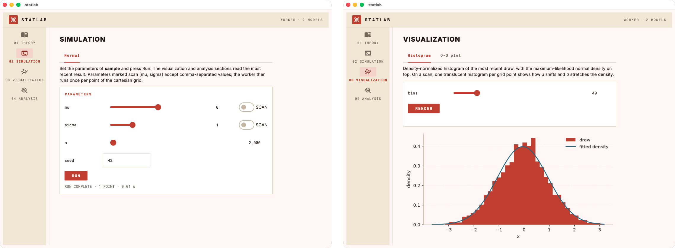
That is the whole app. lab.open() serves it at http://127.0.0.1:8600 and
opens your browser: one page with four sections — Theory, Simulation,
Visualization, Analysis — a slider for every bounded parameter, a Run button,
and tabs for each registered visualization and analysis. Content keeps a
book-like reading measure, results fade in rather than cut, and every section
is explorable before the first Run.
An extended version of this example lives at
examples/demo_lab.py. It grows the same lab into a
small statistics course: a fitted-density overlay, a Q-Q plot, a likelihood
map drawing joint confidence regions for μ and σ, and an inference tab with
bootstrap confidence intervals, a likelihood ratio test and a Jarque-Bera
normality check — plus a second, gamma-distributed worker whose fit tab sets
the method of moments beside the true maximum-likelihood estimate (Newton's
method, Fisher standard errors), all in plain numpy:
python examples/demo_lab.py                 # serve at http://127.0.0.1:8600
python examples/demo_lab.py --port 8550     # serve at http://127.0.0.1:8550
python examples/demo_lab.py --theme matrix
labforge serve examples/demo_lab.py         # the same thing, from the CLI
Concepts
Worker. One function produces the data. Each keyword argument gets a UI
control from its Param spec — or from the signature default alone, if you
spec nothing:
| spec | control |
|---|---|
Param(default=1.0, bounds=(0, 5)) |
slider with live readout |
Param(kind="int", default=100, bounds=(10, 1000)) |
integer slider |
Param(default=1.0) / "scalar" / "int" |
validated text field |
Param(..., scan=True) / "scalar or array" / "int or array" |
scannable (see below) |
"N-tuple" (e.g. "2-tuple") |
one field per element |
Param(kind="choice", options=["a", "b"]) |
dropdown |
Every Param also takes label= to rename its control and help= for a
tooltip on the control's label. Pressing Enter in any text field runs the
section it belongs to, and an entry that fails to parse flags the field while
the last good value stays live.
Validation happens at registration: unknown spec keys, defaults outside
bounds, or a scan spec on a non-worker function raise ValueError when the
app is assembled, never mid-use.
Parameter scans. A kwarg declared scan=True gets a scan toggle (bounded)
or a comma-separated field (unbounded). Enter 0, 1, 2 and labforge calls the
worker once per point of the cartesian grid across all scanned parameters —
the worker itself always receives scalars. A long scan reports its progress in
the status line as the grid fills in. Downstream functions then receive a
ScanResult: a list of (params, result) records with keys, values() and
axis(name) helpers, distinguished with isinstance(data, ScanResult).
Visualizations. Functions viz(data, **kwargs) returning a matplotlib
figure (bare or (fig, ax)). Each gets a tab with its own controls and a
Render button. Figures are yours — labforge only serializes them; the house
style (labforge.style(fig, ax)) is strictly opt-in.
Analyses. Functions analysis(data, **kwargs) — the return shape picks
the rendering:
| return | rendered as |
|---|---|
dict |
two-column quantity/value table |
list of dicts, or a DataFrame |
full table |
str |
markdown |
Figure or (fig, ax) |
image |
| anything else | its repr |
Multiple workers. Call add_worker more than once for a lab with several
workers. Each worker keeps its own workspace — its controls, its last result and
its per-tab settings — and the add_viz / add_analysis calls after each
add_worker attach that worker's own tabs, so switching workers and back
restores exactly what was there. Several workers need a way to choose among them
(checked when the app is served): a selects_worker model selector, or
worker_view="tabs" to lay the workers out as Simulation tabs.
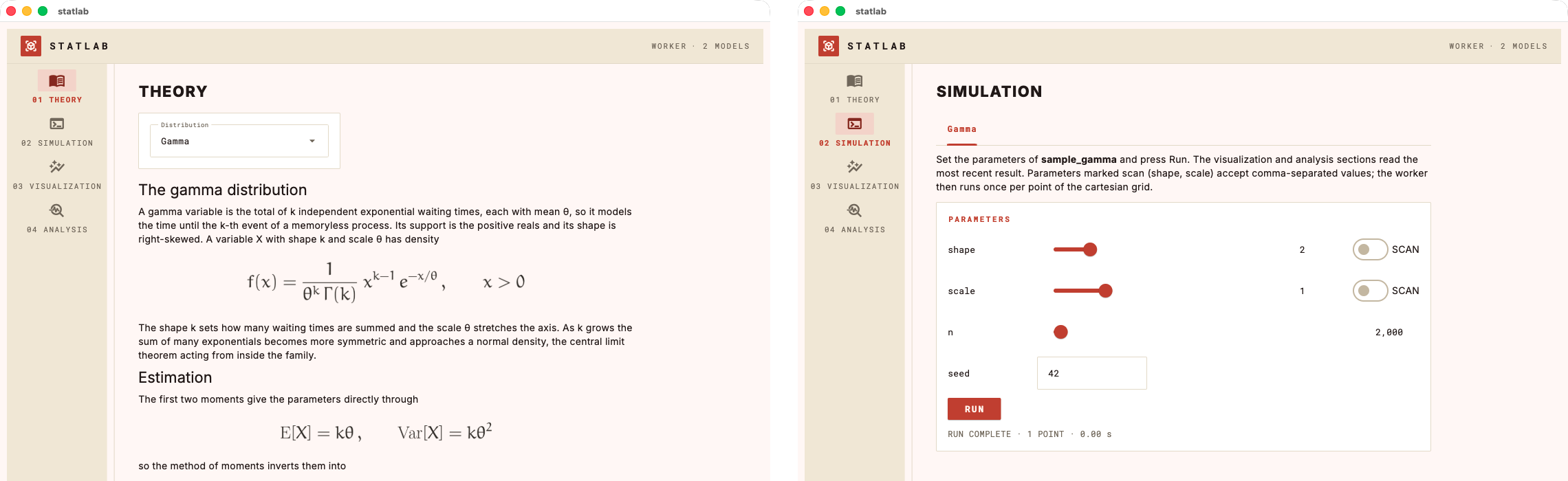
The clean way is a Theory selector with selects_worker=True: its options name
the workers, so choosing one both swaps the theory and makes that worker
active — the Simulation, Visualization and Analysis sections all follow it,
showing only that worker's controls and tabs. The demo
(examples/demo_lab.py) uses this to switch between a normal and a gamma
model:
lab.set_theory_selector(
    "model",
    Param(kind="choice", options=["Normal", "Gamma"]),
    theory_for,                 # theory_for(selection) -> markdown
    label="Distribution",
    selects_worker=True,
)
lab.add_worker(sample, {...}, name="Normal")   # its own viz/analysis tabs
lab.add_worker(sample_gamma, {...}, name="Gamma")
Theory. A markdown file or string. Displayed $$...$$ equations are
typeset in the browser with KaTeX.
Serving and themes
lab.open() takes four independent arguments:
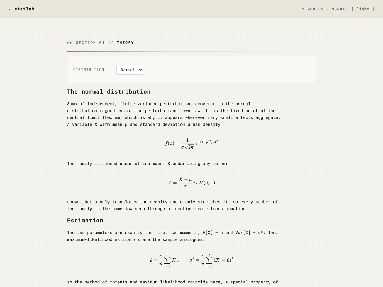
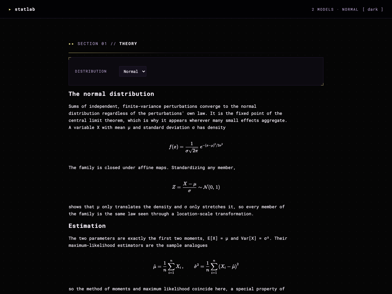
port(default8600) andhost(default127.0.0.1) — with a fixed port the URL is stable across restarts, and every browser tab gets its own isolated session.open_browser— set itFalseto serve without opening a browser.theme— one of three palettes. A theme sets the chrome and the plot palette together, so figures never drift from the app around them. Colour your own figures withlabforge.palette().data,.model,.highlight; list the options withlabforge.themes():
| name | mode | look |
|---|---|---|
light |
light | blue on warm paper white, darkened gold counterpoint (default) |
dark |
dark | terminal-dashboard gold on near-black, violet counterpoint |
matrix |
dark | phosphor terminal green on near-black |
The Theory section in each theme — the equations render with KaTeX:
light |
dark |
matrix |
|---|---|---|
 |
 |
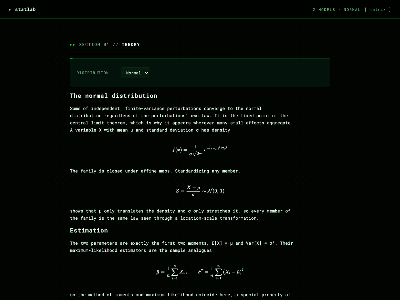 |
The command line
A lab file needs no launch code of its own:
labforge serve mylab.py
serve executes the file (its if __name__ == "__main__" block stays cold, so
it will not start a second server), finds the module-level Lab, and serves it
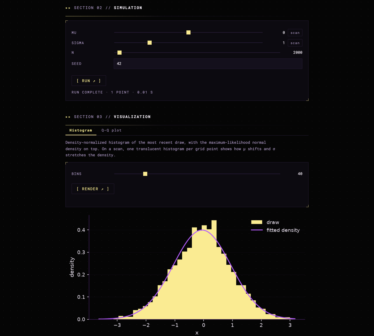
at http://127.0.0.1:8600 — one page, four sections, in a terminal-dashboard
style. Equations render with KaTeX, scans stream RUNNING · k/N progress live
with a thin progress bar, every browser session keeps its own workspace, and a
theme button in the header cycles the palettes, re-rendering open figures so
the plots always match the chrome. Section links in the sticky header track
your scroll, slider readouts accept typed exact values, a scan's comma list
shows its point count as you type, figures open full-size on click, and
analysis tables download as CSV. Pick a theme with --theme, the port with
--port, and pass --no-browser to serve without opening one.
The lab itself is available as data too: lab.to_spec() returns the whole
registration — params, tabs, theory markdown — as one JSON-safe dict, which is
also what the server publishes at /api/spec.
The server binds to localhost by design: a lab is your own Python code, so it is served the way Jupyter serves a notebook — for you, on your machine.
Install
Requires Python ≥ 3.10.
pip install labforge
Or from a clone, if you want to work on the code directly:
git clone https://github.com/laroccod/labforge.git
cd labforge
pip install -e .
Dependencies: fastapi, uvicorn, numpy, matplotlib — that is all.
Equations are typeset in the browser, so no LaTeX toolchain is needed.
Development
pip install -e ".[dev]"
pytest
black --check --line-length 100 src tests examples
The suite runs the server offline over FastAPI's TestClient — the spec
endpoint, a run with its SSE progress stream, viz and analysis payloads, the
generated theme CSS and the error statuses — alongside unit tests for the
registration, scan, dispatch and executor layers, so most mistakes are caught
without serving anything.
License
1 maintainer

Metadata
1 maintainer
Release files for labforge 0.4.0
For a detailed explanation of source distributions (sdists) and built distributions (wheels), please see the package formats documentation.
Source distribution (sdist)
| File | Size | Uploaded | Provenance | Actions |
|---|---|---|---|---|
| labforge-0.4.0.tar.gz | 2.0 MB | Without provenance | Details for labforge-0.4.0.tar.gz |
Built distribution (wheel)
| File | Interpreter | ABI | Platform | Actions Reset |
|---|---|---|---|---|
| labforge-0.4.0-py3-none-any.whl | Python 3 | none | any | Details for labforge-0.4.0-py3-none-any.whl |
Total release size: 2.6 MB
Release files / labforge-0.4.0.tar.gz
| Download URL | labforge-0.4.0.tar.gz |
|---|---|
| Size | 2.0 MB |
| Tags | Source |
|
SHA-256 checksum How to use checksums |
6c406c817f45cb7bc8fb1f7dc0157a11a13beb78662142f033e2bc696ee5c0b8
|
|
BLAKE2b-256 checksum How to use checksums |
5e95b759333a56fe7433bb8146324ba88b168aa6062d2a36eb4d3f60ca756bd7
|
| Upload date | |
|
Uploaded using Trusted Publishing? What is trusted publishing? |
No |
| Uploaded via |
twine/7.0.0 CPython/3.12.13
|
Release files / labforge-0.4.0-py3-none-any.whl
| Download URL | labforge-0.4.0-py3-none-any.whl |
|---|---|
| Size | 637.9 kB |
| Tags | Python 3 |
|
SHA-256 checksum How to use checksums |
7ccfbefea67f63fde9e72d21ce83657c490a276d3dc76494251ea8def76d04da
|
|
BLAKE2b-256 checksum How to use checksums |
50e6cc5a2303abf4b3bb22a77cbae076c969ba72985d76c95c2d33288e1f0fd6
|
| Upload date | |
|
Uploaded using Trusted Publishing? What is trusted publishing? |
No |
| Uploaded via |
twine/7.0.0 CPython/3.12.13
|
Security for labforge 0.4.0
Provenance
Provenance describes where a file came from. On PyPI, provenance is shared via attestations, which provide a verifiable record of the build or publishing details. View details, limitations and caveats.
No provenance found
None of the files in this release were uploaded with provenance metadata.
A note on package security
PyPI is a repository for distributing packages, not a service for auditing them. While third-party security researchers and our staff do their best to detect and remove malicious packages, PyPI cannot guarantee the quality, security or suitability of any given package.
To learn more about protecting yourself from malicious actors, visit our package security documentation.














