Package to visualize LLM's Neural Networks activation regions

Project description
LLM-MRI: a brain scanner for LLMs
This repository contains the implementation from the paper LLM-MRI Python module: a brain scanner for LLMs
As the everyday use of large language models (LLMs) expands, so does the necessity of understanding how these models achieve their designated outputs. LLM-MRI focuses on the activations of the feed-forward layers in a transformer-based LLM through the generation, visualization and analysis of NRAGs.
By adopting this approach, the library examines the neuron activations produced by the model for each distinct label. The objective of this library is to contribute to LLM interpretability research, enabling users to explore visualization methods, such as heatmaps and graph representations of the hidden layers' activations in transformer-based LLMs.
This model allows users to explore questions such as:
- How do different categories of text in the corpus activate different neural regions?
- What are the differences between the properties of NRAGs from two distinct categories?
- Are there regions of activation in the model more related to specific aspects of a category?
We encourage you to not only use this toolkit but also to extend it as you see fit.
Index
Instalation
To see LLM-MRI in action on your own data:
pip install llm_mri
Usage
Firstly, the user needs to choose a dimensionality reduction (PCA, SVD or UMAP) algorithm to be used on the model's internal activations.
from llm_mri.dimensionality_reduction import PCA
pca = PCA(n_components,
          random_state,
          gridsize)
gridsize: parameter used to define the size of heatmaps. Those are only available when the number of components is equal to 2.
Then, import the ActivationAreas package, in order to build the NRAGs, and the matplotlib.pyplot package to render its visualizations:
from llm_mri import ActivationAreas
import matplotlib.pyplot as plt
The user also needs to specify the Hugging Face Dataset that will be used to process the model's activations. There are two ways to do this:
- Load the Dataset from Hugging Face Hub:
dataset_url = "https://huggingface.co/datasets/dataset_link" dataset = load_dataset("csv", data_files=dataset_url) - If you already have the dataset loaded on your machine, you can use the load_from_disk function:
dataset = load_from_disk(dataset_path) # Specify the Dataset's path
Make sure that the selected dataset is a HuggingFace Dataset, and contains the columns "text" and "label", the last one being "ClassLabel" type. For more instructions on how to make this conversion, check out some of the examples on the GitHub documentation.
Next, the user selects the model to be used as a string:
model_ckpt = "distilbert/distilbert-base-multilingual-cased"
Then, the user instantiates ActivationAreas, to apply the methods defined later, on the Functions sections:
llm_mri = ActivationAreas(model=model_ckpt,
                          device="cpu",
                          dataset=dataset,
                          reduction_method=pca)
For now, we recommend to use "cpu" as device. Further tests are going to be executed to ensure full "gpu" compatibility.
Functions
The library's functionality is divided into the following sections:
Activation Extraction:
As the user inputs the model and corpus to be analyzed, the dimensionality of the model's hidden layers is reduced accordingly to the dimensionality algorithm previously passed.
llm_mri.process_activation_areas()
Heatmap Representation of Activations:
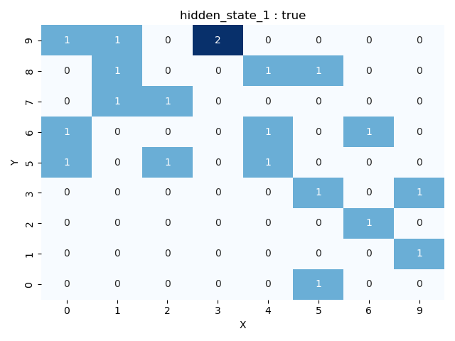
This includes the get_grid function, which transforms the NxN grid for a selected layer into a heatmap (grid). In this heatmap, each cell represents the number of activations that the specific reduced region on a determined layer received for the provided corpus. Additionally, users can visualize activations for a specific label.
Heatmaps can only be obtained if the number of components is set to 2, since all activations are disposed on a 2-dimensional map. Note that for a gridsize of N, N^2 NRAGs are generated, as shown on the grid
fig = llm_mri.get_grid(layer, category)
Graph Representation of Activations:
Using the get_graph function, the module connects regions from neighboring layers based either on the heatmaps (2 dimensions) or through the Spearman Correlation of neighboring layers activations (>2 dimensions). The graph's edges can also be colored according to different labels, allowing the user to identify the specific category that activated each neighboring node.
graph = llm_mri.get_graph(category)
graph_image = llm_mri.get_graph_image(graph, colormap, fix_node_positions)
categories: String or (list of at most two strings) containing the categories that to be used to generate the NRAG.
colormap: The default used colormap is the 'coolwarm'. More can be found on matplotlib.colors. We recommend the use of a 'Diverging' colormap for better visualization.
fix_node_positions: 'True' keeps the nodes and edges at the same positions, independently of the categories. This could be useful for comparing activations between distinct categories. Setting to 'False' does not allow this comparison, although the graph will be more easily visualized.
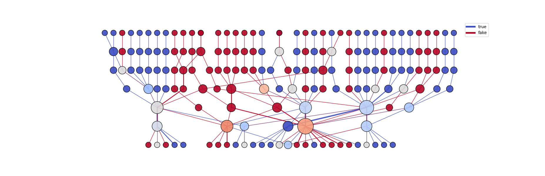
On the graph above (generated with 2D UMAP reduction), each node represents a single activated region on a specific layer. Each height corresponds to a different layer, "higher" nodes being early model layer's activations.
Graph Metrics
The library also provides a set of complex network metrics to be obtained from the generated graphs.
The currently available metrics are mean degree, kurt degree, mean strength, skew strength, assortativity, density and center of mass
metrics = Metrics(graph, model, label)
metrics_dictionary = metrics.get_basic_metrics()
Release history Release notifications | RSS feed


Download files
Download the file for your platform. If you're not sure which to choose, learn more about installing packages.
Source Distribution
Built Distribution
Filter files by name, interpreter, ABI, and platform.
If you're not sure about the file name format, learn more about wheel file names.
Copy a direct link to the current filters
File details
Details for the file llm_mri-0.2.0.tar.gz.
File metadata
- Download URL: llm_mri-0.2.0.tar.gz
- Upload date:
- Size: 23.2 kB
- Tags: Source
- Uploaded using Trusted Publishing? No
- Uploaded via: poetry/1.8.3 CPython/3.9.13 Linux/6.8.0-85-generic
File hashes
| Algorithm | Hash digest | |
|---|---|---|
| SHA256 |
688e35e38d8af54d5c9375a649654203815f5c6a186d004d282b2b924c2d82a8
|
|
| MD5 |
ab34a8f4c99766cb56747d93a1076f00
|
|
| BLAKE2b-256 |
48a8199fe1546dc83a9c8638b352292ebf1733e234ae31358e30132d9ac46318
|
File details
Details for the file llm_mri-0.2.0-py3-none-any.whl.
File metadata
- Download URL: llm_mri-0.2.0-py3-none-any.whl
- Upload date:
- Size: 27.2 kB
- Tags: Python 3
- Uploaded using Trusted Publishing? No
- Uploaded via: poetry/1.8.3 CPython/3.9.13 Linux/6.8.0-85-generic
File hashes
| Algorithm | Hash digest | |
|---|---|---|
| SHA256 |
dee3151746be66413a63410fdc61e3868bdda86fc3667c5c5eb21364850afa1d
|
|
| MD5 |
a85713e7fcf215e341628388f74553e4
|
|
| BLAKE2b-256 |
f8125da6d55041ea9ef725196a8944457e80eddc88272857b6a8eeb9cfd60ad4
|


