

📦 Installation
pip install mannks
Requirements: Python 3.7+, NumPy, Pandas, SciPy, Matplotlib, Piecewise-Regression
✨ What is MannKS?
MannKS (Mann-Kendall Sen) is a Python package for detecting trends in time series data using non-parametric methods. It's specifically designed for environmental monitoring, water quality analysis, and other fields where data is messy, irregular, or contains detection limits.
When to Use MannKS
Use this package when your data has:
- Irregular sampling intervals (daily → monthly → quarterly)
- Censored values (measurements like
<5or>100) - Seasonal patterns you need to account for
- No normal distribution (non-parametric methods don't require it)
- Small to large sample sizes (Automatic support for n > 10,000)
NEW IN V0.5.0: Large Dataset Support. MannKS now automatically handles datasets with 10,000+ observations (up to 50,000+) by switching to optimized stochastic algorithms ("Fast Mode") for Sen's slope and using stratified sampling for seasonal tests. This reduces computation time from minutes to seconds while preserving statistical validity. See Example 35 and the Large Dataset Guide.
# Automatic mode handles large data
result = trend_test(x_large, t_large) # Uses fast approximation if n > 5000

# Or force a specific mode
result = trend_test(x, t, large_dataset_mode='fast', max_pairs=100000)
NEW IN V0.4.0: Segmented Trend Analysis. The segmented_trend_test function performs a hybrid segmented regression analysis. It uses Piecewise Regression (OLS) to automatically identify structural breakpoints in the time series, followed by robust Mann-Kendall / Sen's Slope estimation on each identified segment. This allows you to detect distinct phases in a trend (e.g., "Stable" -> "Rapid Decrease" -> "Stable").
NEW IN V0.3.0: Rolling Trend Analysis. The rolling_trend_test function allows you to perform a rolling window analysis, calculating the Sen's slope, Mann-Kendall score, and confidence intervals over time. This enables the detection of when a trend started, stopped, or changed direction, rather than just providing a single global summary. The feature includes:
- Flexible window sizes (numeric or time-based, e.g., '10 years')
compare_periodsutility to statistically test for changes in trend between two time periods (e.g., before vs. after an intervention).
NEW IN V0.2.0: The trend_test and seasonal_trend_test functions now support a Block Bootstrap method (autocorr_method='block_bootstrap'). This feature provides robust trend testing for data with serial correlation (autocorrelation) by resampling blocks of data rather than individual points, preserving the internal dependency structure.
See Statistical Methodology: Bootstrap for a detailed explanation of the hybrid methodology:
- Hypothesis Testing (P-values): Uses Detrended Residual Block Bootstrap to generate a null distribution while preserving autocorrelation.
- Confidence Intervals (Sen's Slope): Uses Pairs Block Bootstrap to avoid bias when "reconstructing" censored data values from residuals.
Performance (v0.5.0)
| Dataset Size | Mode | Time | Accuracy |
|---|---|---|---|
| 1,000 | Full | 0.1s | Exact |
| 5,000 | Full | 2s | Exact |
| 10,000 | Fast | 3s | ±0.5% |
| 50,000 | Fast | 5s | ±0.5% |
| 100,000 | Aggregate* | 10s | Depends** |
* Aggregate to ~1000 points first ** Accuracy depends on aggregation method and trend pattern
🚀 Quick Start
import pandas as pd
from MannKS import prepare_censored_data, trend_test

# 1. Prepare data with censored values
# Converts strings like '<5' into a structured format
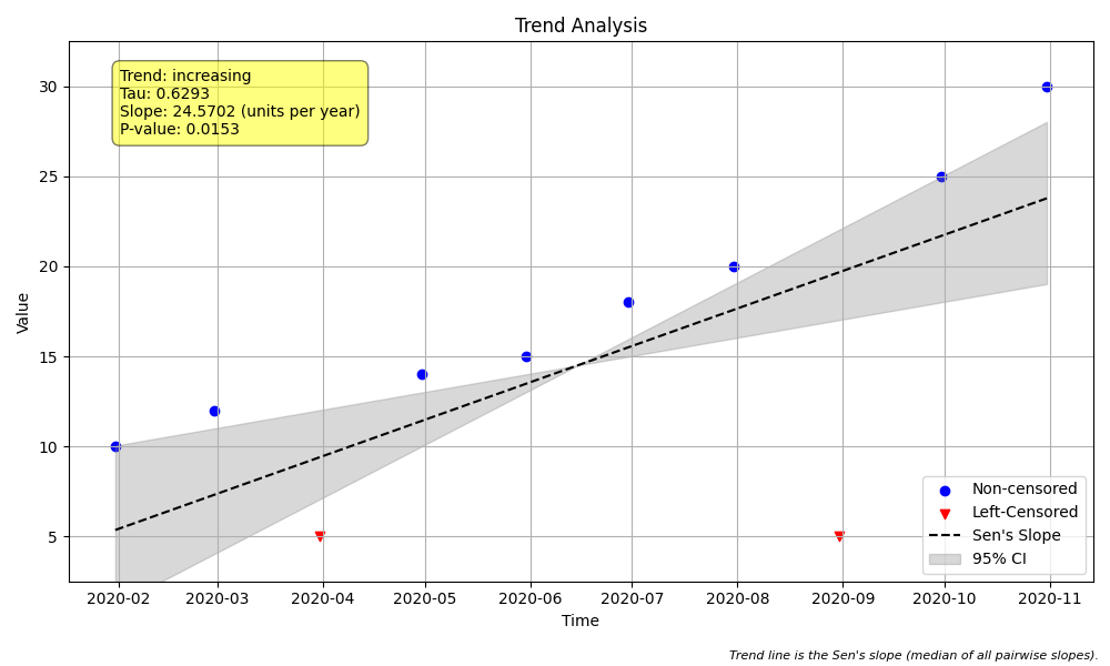
values = [10, 12, '<5', 14, 15, 18, 20, '<5', 25, 30]
dates = pd.date_range(start='2020-01-01', periods=len(values), freq='ME')
data = prepare_censored_data(values)

# 2. Run trend test
# slope_scaling converts slope from "per second" to "per year"
result = trend_test(
    x=data,
    t=dates,
    slope_scaling='year',
    x_unit='mg/L',
    plot_path='trend.png'
)

# 3. Interpret results
print(f"Trend: {result.classification}")
print(f"Slope: {result.slope:.2f} {result.slope_units}")
print(f"Confidence: {result.C:.2%}")
Output:
Trend: Highly Likely Increasing
Slope: 24.57 mg/L per year
Confidence: 98.47%
🎯 Key Features
Core Functionality
- Mann-Kendall Trend Test: Detect monotonic trends with statistical significance
- Sen's Slope Estimator: Calculate trend magnitude with confidence intervals
- Seasonal Analysis: Separate seasonal signals from long-term trends
- Regional Aggregation: Combine results across multiple monitoring sites
Data Handling
- Censored Data Support: Native handling of detection limits (
<5,>100)- Three methods: Standard, LWP-compatible, Akritas-Theil-Sen (ATS)
- Handles left-censored, right-censored, and mixed censoring
- Unequal Spacing: Uses actual time differences (not just rank order)
- Missing Data: Automatically handles NaN values and missing seasons
- Temporal Aggregation: Multiple strategies for high-frequency data
- Large Dataset Support: Optimized algorithms for N > 10,000 (New in v0.5.0)
Statistical Features
- Continuous Confidence: Reports likelihood ("Highly Likely Increasing") not just p-values
- Data Quality Checks: Automatic warnings for tied values, long runs, insufficient data
- Robust Methods: ATS estimator for heavily censored data
- Flexible Testing: Kendall's Tau-a or Tau-b, custom significance levels
- Rolling Trends (New in v0.3.0): Analyze how trends evolve over time with
rolling_trend_test. See Example 31. - Segmented Trends (New in v0.4.0): Automatically detect breakpoints and analyze trends in segments with
segmented_trend_test. See Example 32. - Block Bootstrap (New in v0.2.0): Robust trend testing for autocorrelated data with automatic ACF-based block size selection. See bootstrap.md for details and Example 29.
📊 Example Use Cases
Seasonal Water Quality Trend
from MannKS import seasonal_trend_test, check_seasonality

# Check if seasonality exists (period=12 is inferred from season_type='month')
seasonality = check_seasonality(x=data, t=dates, season_type='month')
print(f"Seasonal pattern detected: {seasonality.is_seasonal}")

# Run seasonal trend test
result = seasonal_trend_test(
    x=data,
    t=dates,
    season_type='month',         # Infers period=12 automatically
    agg_method='robust_median',  # Aggregates multiple samples per month
    slope_scaling='year'
)
Regional Analysis Across Sites
from MannKS import regional_test

# Run trend tests for each site
site_results = []
for site in ['Site_A', 'Site_B', 'Site_C']:
    result = trend_test(x=site_data[site], t=dates)
    site_results.append({
        'site': site,
        's': result.s,
        'C': result.C
    })

# Aggregate regional trend
regional = regional_test(
    trend_results=pd.DataFrame(site_results),
    time_series_data=all_site_data,
    site_col='site'
)
print(f"Regional trend: {regional.DT}, confidence: {regional.CT:.2%}")
⚠️ Important Limitations
Sample Size
- Recommended maximum: n = 50,000 (using default Fast Mode)
- Hard limit: n = 46,340 (if using
large_dataset_mode='full') - For larger datasets, use
large_dataset_mode='aggregate'orregional_test()
Statistical Assumptions
- Independence: Data points must be serially independent
- Autocorrelation violates this and causes spurious significance
- Pre-test with ACF or use block bootstrap methods if autocorrelated
- Monotonic trend: Cannot detect U-shaped or cyclical patterns
- Homogeneous variance: Most powerful when variance is constant over time
📚 Documentation
Detailed Guides
- Trend Test Parameters - Full parameter reference
- Seasonal Analysis - Season types and aggregation
- Regional Tests - Multi-site aggregation
- Analysis Notes - Interpreting data quality warnings
- Trend Classification - Understanding confidence levels
- Bootstrap Methodology - Block bootstrap for autocorrelated data
- Rolling Trend Analysis - Moving window analysis
- Segmented Trend Analysis - Structural breakpoint detection
- Large Dataset Analysis - Fast mode and stratification
Examples
The Examples folder contains step-by-step tutorials from basic to advanced usage.
🔬 Validation
Extensively validated against:
- LWP-TRENDS R script (34 test cases, 99%+ agreement)
- NADA2 R package (censored data methods)
- Edge cases: missing data, tied values, all-censored data, insufficient samples
See validation/ for detailed comparison reports.
🙏 Acknowledgments
This package is heavily inspired by the excellent work of LandWaterPeople (LWP). The robust censored data handling and regional aggregation methods are based on their R scripts and methodologies.
📖 References
- Helsel, D.R. (2012). Statistics for Censored Environmental Data Using Minitab and R (2nd ed.). Wiley.
- Gilbert, R.O. (1987). Statistical Methods for Environmental Pollution Monitoring. Wiley.
- Hirsch, R.M., Slack, J.R., & Smith, R.A. (1982). Techniques of trend analysis for monthly water quality data. Water Resources Research, 18(1), 107-121.
- Mann, H.B. (1945). Nonparametric tests against trend. Econometrica, 13(3), 245-259.
- Sen, P.K. (1968). Estimates of the regression coefficient based on a particular kind of rank correlation. Journal of the American Statistical Association, 63(324), 1379-1389.
- Fraser, C., & Whitehead, A. L. (2022). Continuous measures of confidence in direction of environmental trends at site and other spatial scales. Environmental Challenges, 9, 100601.
- Fraser, C., Snelder, T., & Matthews, A. (2018). State and trends of river water quality in the Manawatu-Whanganui region. Report for Horizons Regional Council.
1 maintainer

Metadata
1 maintainer
Release files for mannks 0.5.0
For a detailed explanation of source distributions (sdists) and built distributions (wheels), please see the package formats documentation.
Source distribution (sdist)
| File | Size | Uploaded | |
|---|---|---|---|
| mannks-0.5.0.tar.gz | 73.0 kB | Details |
Built distribution (wheel)
| File | Interpreter | ABI | Platform | Reset |
|---|---|---|---|---|
| mannks-0.5.0-py3-none-any.whl | Python 3 | none | any | Details |
Total release size: 157.7 kB
Release files / mannks-0.5.0.tar.gz
| Download URL | mannks-0.5.0.tar.gz |
|---|---|
| Size | 73.0 kB |
| Tags | Source |
|
SHA-256 checksum How to use checksums |
a8d9042ed274abd8e6a4b3235c3a08c43fb77ebb70ab621ca584e9abad2b308d
|
|
BLAKE2b-256 checksum How to use checksums |
882461553010f1da4c89ebc617768649334086d06caa6c02556afcee5355e698
|
| Upload date | |
|
Uploaded using Trusted Publishing? What is trusted publishing? |
No |
| Uploaded via |
poetry/1.7.1 CPython/3.10.6 Linux/4.15.0-142-generic
|
Release files / mannks-0.5.0-py3-none-any.whl
| Download URL | mannks-0.5.0-py3-none-any.whl |
|---|---|
| Size | 84.6 kB |
| Tags | Python 3 |
|
SHA-256 checksum How to use checksums |
9ceb742ea44c3cc10218f43aa6519f8f6d4f5d53e79f10b0445157c452b9ae0b
|
|
BLAKE2b-256 checksum How to use checksums |
d107d9d04e31be4eccc6cc223bdf39aad4e13f0d6ce0a38e2719538596ad1f44
|
| Upload date | |
|
Uploaded using Trusted Publishing? What is trusted publishing? |
No |
| Uploaded via |
poetry/1.7.1 CPython/3.10.6 Linux/4.15.0-142-generic
|














