
Classic stock charts in Python
Create classic technical analysis stock charts in Python with minimal code.
The library is built around matplotlib
and supports both pandas
and polars DataFrames.
Charts can be defined using a declarative interface,
based on a set of drawing primitives like Candlesticks, Volume
and technical indicators like SMA, EMA, RSI, ROC, MACD, etc ...
📖 Documentation: tutorials, API reference and a chart gallery at furechan.github.io/mplchart
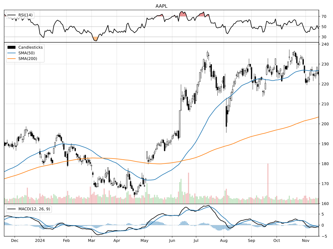
Typical usage
# Candlesticks chart with SMA, RSI and MACD indicators

import yfinance as yf

from mplchart.chart import Chart
from mplchart.primitives import Candlesticks, Volume, Pane, Line
from mplchart.indicators import SMA, RSI, MACD

ticker = 'AAPL'
prices = yf.Ticker(ticker).history('5y')

Chart(prices, title=ticker, max_bars=250, normalize=True).plot(
    Candlesticks(), Volume(), SMA(50), SMA(200),
    Pane("above", yticks=(30, 50, 70)),
    RSI(14) @ Line(overbought=70, oversold=30),
    Pane("below"),
    MACD(),
).show()
SMA and MACD use default rendering. The @ operator binds RSI(14) to a Line renderer to customize its display; Line(RSI(14), ...) is the equivalent constructor form.
Plotting indicators
Pass indicators directly to plot() to calculate values from prices during plotting and use default rendering. For example, SMA(20) computes a moving average and draws it as a line; no renderer primitive is required. With polars data, import the factories from mplchart.expressions instead of mplchart.indicators.
from mplchart.chart import Chart
from mplchart.samples import sample_prices
from mplchart.primitives import Candlesticks
from mplchart.indicators import SMA

prices = sample_prices(backend="pandas")

Chart(prices, max_bars=250).plot(
    Candlesticks(),
    SMA(20),
).show()
To customize the display, optionally use a renderer such as Line, Area, or Bars: Line(SMA(20), color="red") draws the moving average in red. SMA(20) @ Line(color="red") is an equivalent binding form; both defer calculation until plotting. Parenthesize composed expressions before binding, for example (EMA(20) - EMA(50)) @ Area() with polars expressions. Pandas expressions (pd.col(...) or .as_expr()) require constructor binding because pandas handles @ itself.
If your data pipeline already adds custom columns to prices, you can also plot those by name alongside the price data: Chart(prices).plot(Candlesticks(), "sma-20") reads the existing sma-20 column and uses default line rendering. Use Line("sma-20", color="red") to customize its appearance.
Styles
Charts are styled via the style= option — a builtin style, any matplotlib stylesheet name, or a custom style dict. Styles are total: ambient matplotlib settings never affect a chart.
from mplchart.styles import available_styles

available_styles()
# ['chartist', 'modern', 'mplchart', 'nightclouds']

# builtin style
Chart(prices, title=ticker, style="nightclouds").plot(Candlesticks()).show()

# any matplotlib stylesheet
Chart(prices, title=ticker, style="ggplot").plot(Candlesticks()).show()

# custom style dict
MY_STYLE = {
    "stylesheet": "dark_background",
    "settings": {
        "candle.up.color": "#26a69a",
        "candle.down.color": "#ef5350",
    },
}
Chart(prices, title=ticker, style=MY_STYLE).plot(Candlesticks()).show()
Conventions
Prices data is expected to be a dataframe with columns open, high, low, close, volume in lower case and a datetime column named date or datetime (or a datetime index for pandas).
If your data has column names in different capitalization (like data from yfinance) use the normalize option Chart(..., normalize=True) or call normalize_prices explicitely to normalize the dataframe.
# Normalize prices to lower case column names

import yfinance as yf
from mplchart.utils import normalize_prices

prices = normalize_prices(yf.Ticker(ticker).history('5y'))
Drawing primitives
The library contains drawing primitives that can be used like an indicator in the plot api. Primitives are classes and must be instantiated as objects before being used with the plot api.
# Candlesticks chart

from mplchart.chart import Chart
from mplchart.primitives import Candlesticks

Chart(prices, title=title, max_bars=250).plot(
    Candlesticks()
).show()
The main drawing primitives are :
Candlesticksfor candlestick plotsHeikinAshifor Heikin-Ashi candle plotsRenkofor Renko brick plots (time-independent bricks of fixed price size)PointFigurefor Point & Figure plots (X/O columns on a box grid)OHLCfor open, high, low, close bar plotsVolumefor volume bar plotsPaneto open a new pane (above or below) for the primitives that followLinedraw a column, indicator, or expression as a line plotAreadraw a column, indicator, or expression as a area plotBarsdraw a column, indicator, or expression as a bar plotBandsdraw upper/lower(/middle) bands with a translucent fillStripesto shade background areas where a condition is activeMarkersto mark signal crossings with symbolsZigZaglines between pivot pointsSwingsto mark local peaks and valleys (swing highs/lows)TrendLinesto fit support and resistance trend lines (experimental)HLineto draw a horizontal reference line on the current paneVLineto draw a vertical line across all panes at a given date
Builtin indicators
The library includes some standard technical analysis indicators for pandas DataFrames.
Indicators are classes and must be instantiated as objects before being used with the plot api.
Instantiated they are callables, you can apply them like calling a function SMA(50)(prices).
Some of the indicators included are:
SMASimple Moving AverageEMAExponential Moving AverageWMAWeighted Moving AverageHMAHull Moving AverageRMARolling Moving Average (Wilder's)DEMADouble Exponential Moving AverageTEMATriple Exponential Moving AverageMOMMomentumROCRate of ChangeRSIRelative Strength IndexADXAverage Directional IndexDMIDirectional Movement IndexMACDMoving Average Convergence DivergencePPOPrice Percentage OscillatorBOPBalance of PowerCMFChaikin Money FlowMFIMoney Flow IndexSTOCHStochastic OscillatorTRANGETrue RangeATRAverage True RangeNATRNormalized Average True RangeBBANDSBollinger BandsBBPBollinger Bands PercentBBWBollinger Bands WidthKELTNERKeltner ChannelDONCHIANDonchian ChannelMEDPRICEMedian PriceTYPPRICETypical PriceWCLPRICEWeighted Close PriceAVGPRICEAverage Price
Pass an indicator to a rendering primitive to customize display — the @ binding operator is an equivalent alternative:
# Customizing indicator style with Line

from mplchart.indicators import SMA, EMA, ROC
from mplchart.primitives import Candlesticks, Line

indicators = [
    Candlesticks(),
    Line(SMA(20), style="dashed", color="red", alpha=0.5, width=3)
]

Chart(prices).plot(indicators)
Polars expressions
For polars DataFrames, the expressions subpackage provides polars Expr factories
as an alternative to the indicator pattern.
These can be used directly with chart.plot().
# Candlesticks chart with polars expressions

from mplchart.chart import Chart
from mplchart.primitives import Candlesticks, Volume, Pane, Line
from mplchart.expressions import SMA, EMA, RSI, MACD

Chart(prices, title=ticker, max_bars=250).plot(
    Candlesticks(), Volume(),
    SMA(50).alias("sma50"), SMA(200).alias("sma200"),
    Pane("above", yticks=(30, 50, 70)),
    Line(RSI(), overbought=70, oversold=30),
    Pane("below"),
    MACD(),
).show()
Expressions are plain polars.Expr values — they can be composed with standard polars operators,
passed to df.select(), or used anywhere polars expressions are accepted.
Pass an expression to a rendering primitive to customize display — the @ binding operator is an equivalent alternative:
from mplchart.primitives import Line, Area
from mplchart.expressions import SMA, RSI

Line(SMA(50), color="red")     # expression → primitive
Area(RSI(14), color="blue")    # expression → primitive
SMA(50) @ Line(color="red")    # operator form
TA-Lib functions
If you have TA-Lib installed you can use its abstract functions as indicators. They are created by calling the Function factory with the name of the function and its parameters. TA-Lib functions work with both pandas and polars backends.
# Candlesticks chart with talib functions

from mplchart.primitives import Candlesticks
from talib.abstract import Function

indicators = [
    Candlesticks(),
    Function('SMA', 50),
    Function('SMA', 200),
]

Chart(prices).plot(indicators).show()
Third-party indicators
mintalib provides additional technical analysis indicators. Pass them directly to plot() for default rendering. Its imports follow the same backend convention as mplchart: indicators for pandas and expressions for polars. Install mintalib separately, then choose the import matching your prices DataFrame.
For pandas data:
from mintalib.indicators import CCI
For polars data:
from mintalib.expressions import CCI
With prices in the corresponding backend, the chart code is the same. Draw CCI in its own pane below the price chart:
from mplchart.chart import Chart
from mplchart.primitives import Candlesticks

Chart(prices, max_bars=250).plot(
    Candlesticks(),
).pane("below").plot(
    CCI(20),
).show()
Calculations are deferred until plotting and use default rendering. Optional renderer binding works too: Line(CCI(20), color="red") or CCI(20) @ Line(color="red").
Examples
Example notebooks live in the examples folder and render as tutorials on the documentation site at furechan.github.io/mplchart.
Installation
pip install mplchart
The indicators module requires pandas; the expressions module requires polars.
If either is already in your environment, mplchart will use it automatically.
The [pandas], [polars], and [all] extras are just a convenience — they
install pandas or polars alongside mplchart, nothing more:
pip install mplchart[pandas]
pip install mplchart[polars]
pip install mplchart[all]
Notebook chart widget
Install the notebook extra alongside your chosen data backend:
pip install 'mplchart[notebook,pandas]'
Pass a callable that accepts a ticker and returns a prices DataFrame. The widget displays centered Ticker and Max bars inputs above the chart:
from mplchart.notebook import chart_widget

chart_widget(get_prices, ticker="AAPL", max_bars=250)
The default chart shows candlesticks and volume. Pass indicators=[Candlesticks(), SMA(50), Volume()] to supply the complete plot sequence, or chart options such as style="nightclouds", figsize=(12, 8), and normalize=True. Match pandas indicators or Polars expressions to your loader's backend.
A bardata feed works directly as chart_widget(feed.get, ticker="AAPL"). Use functools.partial(feed.get, freq="weekly") to bind loader options. mplchart does not require bardata or any other data provider.
Max bars changes only the visible window and reuses the current ticker's loaded history, preserving indicator warm-up. Switching tickers calls the loader again; data caching belongs to the loader. The returned widget displays as the last expression in a notebook cell, or via display(widget), and requires a live kernel with widget support.
Dependencies
Required:
- python >= 3.10
- matplotlib
- numpy
- pyarrow
Optional extras:
[pandas]— pandas[polars]— polars[all]— pandas and polars[notebook]— ipywidgets and IPython formplchart.notebook.chart_widget
Related projects
- mplfinance - Matplotlib utilities for the visualization, and visual analysis, of financial data
- matplotlib - Matplotlib: plotting with Python
- morethemes - More themes for matplotlib
- pandas - Flexible and powerful data analysis / manipulation library for Python
- polars - Fast DataFrame library for Python
- ta-lib - Python wrapper for TA-Lib
- mintalib - Technical analysis indicators for Python
- yfinance - Download market data from Yahoo! Finance's API
1 maintainer

Release files for mplchart 0.0.54
For a detailed explanation of source distributions (sdists) and built distributions (wheels), please see the package formats documentation.
Built distribution (wheel)
| File | Interpreter | ABI | Platform | Reset |
|---|---|---|---|---|
| mplchart-0.0.54-py3-none-any.whl | Python 3 | none | any | Details |
Release files / mplchart-0.0.54-py3-none-any.whl
| Download URL | mplchart-0.0.54-py3-none-any.whl |
|---|---|
| Size | 646.4 kB |
| Tags | Python 3 |
|
SHA-256 checksum How to use checksums |
8a8982ecd35123b0e1493c91c81a0e2aa17f459daa8667380d7d3fae773a053e
|
|
BLAKE2b-256 checksum How to use checksums |
d94db40aa6dc333d92e8f6ec8c7ac8a60a71d336326ed934d8c897e7d6cd3a06
|
| Upload date | |
|
Uploaded using Trusted Publishing? What is trusted publishing? |
Yes |
| Uploaded via |
uv/0.12.17 {"installer":{"name":"uv","version":"0.12.17","subcommand":["publish"]},"python":null,"implementation":{"name":null,"version":null},"distro":{"name":"Ubuntu","version":"24.04","id":"noble","libc":null},"system":{"name":null,"release":null},"cpu":null,"openssl_version":null,"setuptools_version":null,"rustc_version":null,"ci":true}
|














