multimin 0.10.4

MultiMin: Multivariate Gaussian fitting

Introducing MultiMin

MultiMin is a Python package designed to provide numerical tools for fitting data to a Mixture of Gaussians (MoG, see below). It can process a sample of \(n\) variables to find the set of multivariate normal distributions that best describe the data. Additionally, the package can fit one-dimensional data (e.g., numerical functions, time-series, etc.) to a composition of Gaussians.

These are the main features of MultiMin:

• Multivariate Normal Distributions: Define, plot, and sample single or mixture of gaussians.

• Multivariate Data Visualization: Visualize multivariate datasets using corner plots, scatter diagrams, and density plots.

• Multivariate Data Fitting: Fit multivariate data to Mixtures of Gaussians (MoG), including one-dimensional data such as time-series, numerical functions, and spectra.

Resources

• Examples and API documentation: https://multimin.readthedocs.io.

• PyPI project page: https://pypi.org/project/multimin/.

• Github repo: https://github.com/seap-udea/multimin

Installation

From PyPI

MultiMin is available on PyPI at https://pypi.org/project/multimin/. You can install it with:

pip install -U multimin

If you prefer, you can install the latest version of the developers taking it from the github repo:

pip install -U git+https://github.com/seap-udea/multimin

Theoretical Background: the MoG

The core of MultiMin is the Mixture of Gaussians (MoG) defined as:

\begin{equation*} \mathcal{C}_{M,k}(\tilde U; \{w_k\}_M, \{\mu_k\}_M, \{\Sigma_k\}_M) \equiv \sum_{i=1}^{M} w_i\mathcal{N}_k(\tilde U; \tilde \mu_i, \Sigma_i) \end{equation*}

where \(\tilde U:(u_1,u_2,u_3,\ldots,u_N)\) are random variables and the multivariate normal distribution (MND) \(\mathcal{N}_k(\tilde U; \tilde \mu, \Sigma)\) with mean vector \(\tilde \mu\) and covariance matrix \(\Sigma\) is given by:

\begin{equation*} \mathcal{N}_k(\tilde U; \tilde \mu, \Sigma) = \frac{1}{\sqrt{(2\pi)^{k} \det \Sigma}} \exp\left[-\frac{1}{2}(\tilde U - \tilde \mu)^{\rm T} \Sigma^{-1} (\tilde U - \tilde \mu)\right] \end{equation*}

The covariance matrix \(\Sigma\) elements are defined as \(\Sigma_{ij} = \rho_{ij}\sigma_{i}\sigma_{j}\), where \(\sigma_i\) is the standard deviation of \(u_i\) and \(\rho_{ij}\) is the correlation coefficient between variable \(u_i\) and \(u_j\) (\(-1<\rho_{ij}<1\), \(\rho_{ii}=1\)).

The normalization condition implies that the set of weights \(\{w_k\}_M\) are also normalized, i.e., \(\sum_i w_i=1\).

Quickstart

Getting started with MultiMin is straightforward. Import the package:

import multimin as mn

NOTE: If you are working in Google Colab, load the matplotlib backend before producing plots:

%matplotlib inline

Here is a basic example of how to use MultiMin to fit a 3D distribution composed of 2 Multivariate Normals.

1. Define a true distribution

First, we define a distribution from which we will generate synthetic data. We use a Mixture of Gaussians (MoG) with 2 Gaussian components (ngauss=2) in 3 dimensions (nvars=3).

import numpy as np
import multimin as mn

# Define parameters for 2 Gaussian components
weights = [0.5, 0.5]
mus = [[1.0, 0.5, -0.5], [1.0, -0.5, +0.5]]
sigmas = [[1, 1.2, 2.3], [0.8, 0.2, 3.3]]
deg = np.pi/180
angles = [
    [10*deg, 30*deg, 20*deg],
    [-20*deg, 0*deg, 30*deg],
]

# Calculate covariance matrices from rotation angles
Sigmas = mn.Stats.calc_covariance_from_rotation(sigmas, angles)

# Create the MoG object
MoG = mn.MixtureOfGaussians(mus=mus, weights=weights, Sigmas=Sigmas)

2. Generate sample data

We generate 5000 random samples from this distribution to serve as our “observed” data.

np.random.seed(1)
sample = MoG.rvs(5000)

3. Visualize the data

We can check the distribution of the generated data using DensityPlot.

import matplotlib.pyplot as plt

# Define properties labels
properties = dict(
    x=dict(label=r"$x$", range=None),
    y=dict(label=r"$y$", range=None),
    z=dict(label=r"$z$", range=None),
)

# Plot the density plot
G = mn.MultiPlot(properties, figsize=3)

sargs = dict(s=0.5,edgecolor='None',color='r')
scatter = G.sample_scatter(sample,**sargs)

pargs=dict(cmap='Spectral_r')
pdf = G.mog_pdf(MoG,**pargs)

The same properties dict can be passed to MoG.plot_sample and F.plot_fit via the properties argument for consistent axis labels. You can also pass a simple list of names (e.g. properties=["x","y","z"]); then each name is used as the axis label and range=None.

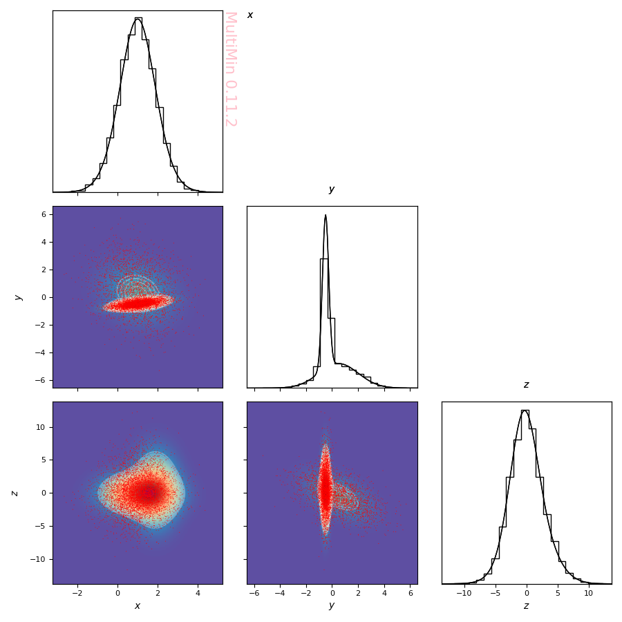
Data Scatter Plot

Theoretical Background: fitting a MoG

The theory behind it posits that any multivariate distribution function \(p(\tilde U):\Re^{N}\rightarrow\Re\), where \(\tilde U:(u_1,u_2,u_3,\ldots,u_N)\) are random variables, can be approximated with arbitrary precision by a normalized linear combination of \(M\) Multivariate Normal Distributions or MoG:

To estimate the parameters of the MoG that best describe a given dataset , we use the Likelihood Statistics method.

Given a dataset of \(S\) objects with state vectors \(\{\tilde U_k\}_{k=1}^S\), the likelihood \(\mathcal{L}\) of the MoG parameters is defined as the product of the probability densities evaluated at each data point:

\begin{equation*} \mathcal{L} = \prod_{i=1}^{S} \mathcal{C}_{M,k}(\tilde U_i) \end{equation*}

The goal is to find the set of parameters (weights, means, and covariances) that maximize this likelihood. In practice, it is numerically more stable to minimize the negative normalized log-likelihood:

\begin{equation*} -\frac{\log \mathcal{L}}{S} = -\frac{1}{S} \sum_{i=1}^{S} \log \mathcal{C}_{M,k}(\tilde U_i) \end{equation*}

This approach allows us to fit the distribution without making strong assumptions about the underlying normality of the data, effectively treating the MoG as a series expansion of the true probability density function.

In MultiMin, we use the scipy.optimize.minimize function to find the set of parameters that minimize the negative normalized log-likelihood.

1. Initialize the Fitter and Run the Fit

We initialize the FitMoG handler with the expected number of Gaussians (2) and variables (3). We then run the fitting procedure.

# Initialize the fitter
F = mn.FitMoG(data=sample, ngauss=2)

# Run the fit (using progress="text" for better convergence on complex models)
F.fit_data(progress="text")

2. Check and Plot Results

Finally, we visualize the fitted distribution compared to the data.

# Plot the fit result (properties accepts the same dict as DensityPlot, or a list of names)
G = F.plot_fit(
    properties=properties,
    pargs=dict(cmap='YlGn'),
    sargs=dict(s=0.2, edgecolor='None', color='r'),
    figsize=3
)

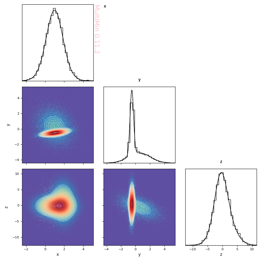
Fit Result

3. Inspect Parameters and Get Explicit PDF Function

You can tabulate the fitted parameters and obtain an explicit Python function that evaluates the fitted PDF. Below, each step is shown with its output.

Stage 1: Tabulate the fitted MoG

F.mog.tabulate(sort_by='weight')

Output:

                  w      mu_1      mu_2      mu_3   sigma_1   sigma_2   sigma_3    rho_12    rho_13    rho_23
component
2          0.509108  1.019245 -0.480997  0.618821  0.794906  0.245786  3.327537  0.539417 -0.008936 -0.017769
1          0.490892  0.957687  0.517584 -0.463392  1.039489  1.538029  2.116544 -0.209695  0.121184 -0.527142

Stage 2: Get the source code and a callable function

code, mog = F.mog.get_function()

Output (the printed code, which you can copy):

from multimin.Util import nmd

def mog(X):

    mu1_1 = 0.957687
    mu1_2 = 0.517584
    mu1_3 = -0.463392
    mu1 = [mu1_1, mu1_2, mu1_3]
    Sigma1 = [[1.080538, -0.335252, 0.266619], [-0.335252, 2.365532, -1.716008], [0.266619, -1.716008, 4.479757]]
    n1 = nmd(X, mu1, Sigma1)

    mu2_1 = 1.019245
    mu2_2 = -0.480997
    mu2_3 = 0.618821
    mu2 = [mu2_1, mu2_2, mu2_3]
    Sigma2 = [[0.631876, 0.10539, -0.023637], [0.10539, 0.060411, -0.014533], [-0.023637, -0.014533, 11.072504]]
    n2 = nmd(X, mu2, Sigma2)

    w1 = 0.490892
    w2 = 0.509108

    return (
        w1*n1
        + w2*n2
    )

Stage 3: Evaluate the PDF at a point

mog([1.0, 0.5, -0.5])

Output:

0.011073778538439395

Stage 4: LaTeX output for papers

You can get the fitted PDF as a LaTeX string (suitable for inclusion in papers) with parameter values and the definition of the normal distribution:

latex_str, _ = F.mog.get_function(print_code=False, type='latex', decimals=4)
print(latex_str)

Output:

\begin{equation*} f(\mathbf{x}) = w_1 \, \mathcal{N}_k(\mathbf{x}; \boldsymbol{\mu}_1, \mathbf{\Sigma}_1) + w_2 \, \mathcal{N}_k(\mathbf{x}; \boldsymbol{\mu}_2, \mathbf{\Sigma}_2) \end{equation*}

where

\begin{equation*} w_1 = 0.4909 \end{equation*}

\begin{equation*} \boldsymbol{\mu}_1 = \left( \begin{array}{c} 0.9577 \\ 0.5176 \\ -0.4634 \end{array}\right) \end{equation*}

\begin{equation*} \mathbf{\Sigma}_1 = \left( \begin{array}{ccc} 1.0805 & -0.3353 & 0.2666 \\ -0.3353 & 2.3655 & -1.716 \\ 0.2666 & -1.716 & 4.4798 \end{array}\right) \end{equation*}

\begin{equation*} w_2 = 0.5091 \end{equation*}

\begin{equation*} \boldsymbol{\mu}_2 = \left( \begin{array}{c} 1.0192 \\ -0.481 \\ 0.6188 \end{array}\right) \end{equation*}

\begin{equation*} \mathbf{\Sigma}_2 = \left( \begin{array}{ccc} 0.6319 & 0.1054 & -0.0236 \\ 0.1054 & 0.0604 & -0.0145 \\ -0.0236 & -0.0145 & 11.0725 \end{array}\right) \end{equation*}

Here the normal distribution is defined as:

\begin{equation*} \mathcal{N}_k(\mathbf{x}; \boldsymbol{\mu}, \mathbf{\Sigma}) = \frac{1}{\sqrt{(2\pi)^{{k}} \det \mathbf{\Sigma}}} \exp\left[-\frac{1}{2}(\mathbf{x}-\boldsymbol{\mu})^{\top} \mathbf{\Sigma}^{{-1}} (\mathbf{x}-\boldsymbol{\mu})\right] \end{equation*}

A parameter table in LaTeX is also available via F.mog.tabulate(sort_by='weight', type='latex').

Truncated multivariate distributions.

In real problems the domain of the variables is not infinite but bounded into a semi-finite region.

If we start from the unbounded multivariate normal distribution:

\begin{equation*} \mathcal{N}_k(\tilde U; \tilde \mu, \Sigma) = \frac{1}{\sqrt{(2\pi)^{k}\det \Sigma}} \exp\left[ -\frac{1}{2}(\tilde U - \tilde \mu)^{\rm T}\Sigma^{-1}(\tilde U - \tilde \mu) \right] \end{equation*}

Let \(T\subset\{l,\dots,m\}\), where \(l\leq k\) and \(m\leq k\) be the set of indices of the truncated variables, and let \(a_i<b_i\) be the truncation bounds for \(i\in T\). Define the truncation region:

\begin{equation*} A_S : \{\tilde U\in\mathbb{R}^k:\ a_i \le \tilde U_i \le b_i \ \ \forall\, i\in T \} \end{equation*}

with the remaining coordinates \(i\notin T\) unbounded. The partially-truncated multivariate normal distribution is defined by

\begin{equation*} \mathcal{TN}_T(\tilde U;\tilde\mu,\Sigma,\mathbf{a}_T,\mathbf{b}_T) = \frac{\mathcal{N}_k(\tilde U;\tilde\mu,\Sigma)\,\mathbf{1}_{A_T}(\tilde U)}{Z_T(\tilde\mu,\Sigma,\mathbf{a}_T,\mathbf{b}_T)}, \end{equation*}

where \(\mathbf{1}_{A_T}\) is the indicator function of \(A_T\) and the normalization constant is

\begin{equation*} Z_T(\tilde\mu,\Sigma,\mathbf{a}_T,\mathbf{b}_T)= \int_{A_T}\mathcal{N}_k(\tilde V;\tilde\mu,\Sigma)\,d\tilde V = \mathbb{P}_{\tilde U\sim\mathcal{N}_k(\tilde\mu,\Sigma)}\left(\tilde U\in A_T\right). \end{equation*}

Example: univariate truncated mixture

Define a mixture of two Gaussians on the interval \([0, 1]\) with the domain parameter, generate data, and fit with FitMoG(..., domain=[[0, 1]]):

import numpy as np
import multimin as mn

# Truncated mixture of 2 Gaussians on [0, 1]
MoG_1d = mn.MixtureOfGaussians(
    mus=[0.2, 0.8],
    weights=[0.5, 0.5],
    Sigmas=[0.01, 0.03],
    domain=[[0, 1]],
)
np.random.seed(1)
data_1d = MoG_1d.rvs(5000)

# Fit with same domain so likelihood and means respect [0, 1]
F_1d = mn.FitMoG(data=data_1d, ngauss=2, domain=[[0, 1]])
F_1d.fit_data(progress="text")
G = F_1d.plot_fit(hargs=dict(bins=40), sargs=dict(s=0.5, alpha=0.6))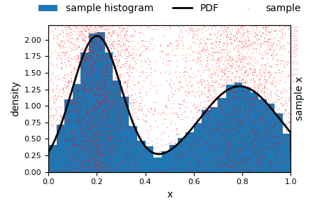

Truncated 1D fit

You can also extract an explicit callable function for the fitted truncated PDF (including the bounds) and evaluate it safely outside the interval.

function, mog = F_1d.mog.get_function()

Output (the printed code, which you can copy):

import numpy as np
from multimin import tnmd

def mog(X):

    a = 0.0
    b = 1.0

    mu1_1 = 0.200467
    sigma1_1 = 0.009683
    n1 = tnmd(X, mu1_1, sigma1_1, a, b)

    mu2_1 = 0.801063
    sigma2_1 = 0.030392
    n2 = tnmd(X, mu2_1, sigma2_1, a, b)

    w1 = 0.504151
    w2 = 0.495849

    return (
        w1*n1
        + w2*n2
    )

Evaluate the fitted PDF at a point inside the domain and outside the domain:

mog(0.5), mog(-0.2)

Output:

(0.3128645172339761, 0.0)

For papers, you can also generate a LaTeX/Markdown description that includes the truncation information:

function_str, _ = F_1d.mog.get_function(print_code=False, type='latex', decimals=4)
print(function_str)

Output:

Finite domain. The following variables are truncated (the rest are unbounded):

• Variable \(x_{1}\) (index 1): domain \([0.0, 1.0]\).

Truncation region: \(A_T = \{\tilde{U} \in \mathbb{R}^k : a_i \le \tilde{U}_i \le b_i \;\forall i \in T\}\), with \(T\) the set of truncated indices.

\begin{equation*} f(x) = w_1 \, \mathcal{TN}(x; \mu_{1}, \sigma_{1}, a, b) + w_2 \, \mathcal{TN}(x; \mu_{2}, \sigma_{2}, a, b) \end{equation*}

where

\begin{equation*} w_1 = 0.5042,\quad \mu_{1} = 0.2005,\quad \sigma_{1}^2 = 0.0097,\quad a = 0.0,\quad b = 1.0 \end{equation*}

\begin{equation*} w_2 = 0.4958,\quad \mu_{2} = 0.8011,\quad \sigma_{2}^2 = 0.0304,\quad a = 0.0,\quad b = 1.0 \end{equation*}

Truncated normal. The unbounded normal is

\begin{equation*} \mathcal{N}_k(x; \mu, \sigma) = \frac{1}{\sigma\sqrt{2\pi}} \exp\left(-\frac{(x-\mu)^2}{2\sigma^2}\right). \end{equation*}

The truncation region is \(A_T = \{\tilde{U} \in \mathbb{R}^k : a_i \le \tilde{U}_i \le b_i \;\forall i \in T\}\). The partially truncated normal is

\begin{equation*} \mathcal{TN}_T(\tilde{U}; \tilde{\mu}, \Sigma, \mathbf{a}_T, \mathbf{b}_T) = \frac{\mathcal{N}_k(\tilde{U}; \tilde{\mu}, \Sigma) \, \mathbf{1}_{A_T}(\tilde{U})}{Z_T(\tilde{\mu}, \Sigma, \mathbf{a}_T, \mathbf{b}_T)}, \end{equation*}

where \(\mathbf{1}_{A_T}\) is the indicator of \(A_T\) and the normalization constant is

\begin{equation*} Z_T(\tilde{\mu}, \Sigma, \mathbf{a}_T, \mathbf{b}_T) = \int_{A_T} \mathcal{N}_k(\tilde{T}; \tilde{\mu}, \Sigma) \, d\tilde{T} = \mathbb{P}_{\tilde{T} \sim \mathcal{N}_k(\tilde{\mu},\Sigma)}(\tilde{T} \in A_T). \end{equation*}

See examples/multimin_truncated_tutorial.ipynb for 3D truncated examples and more detail.

Comparison with scikit-learn

scikit-learn includes a tool for fitting Mixture of Gaussians (known as GMM in that package). While this might seem to overlap significantly with MultiMin, the focus of scikit-learn is primarily on machine learning applications, particularly clustering and Gaussian processes.

MultiMin, on the other hand, was developed with features specifically designed to provide a simplified numerical and analytical description of real physical systems (see for instance this notebook). Additionally, MultiMin extends MoG tools to single-valued functions, a capability with numerous specific applications in physics, astronomy, and other sciences (see for instance this notebook).

For a comparison between MultiMin and scikit-learn GMM, please refer to this notebook.

Citation

The numerical tools and codes provided in this package have been developed and tested over several years of scientific research.

If you use MultiMin in your research, please cite:

@software{multimin2026,
  author = {Zuluaga, Jorge I.},
  title = {MultiMin: Multivariate Gaussian fitting},
  year = {2026},
  url = {https://github.com/seap-udea/multimin}
}

What’s New

For a detailed list of changes and new features, see WHATSNEW.md.

Authors and Licensing

This project is developed by the Solar, Earth and Planetary Physics Group (SEAP) at Universidad de Antioquia, Medellín, Colombia. The main developer is Prof. Jorge I. Zuluaga - [e-mail].

Other beta testers and contributors:

• Juanita A. Agudelo - [e-mail]. Testing of the initial versions of the package in the context of NEAs research. The idea of developíng the functionalities of truncated multinormals were inspared by questions that referees made to Juanita during the presentation of her undergraduate thesis.

This project is licensed under the GNU Affero General Public License v3.0 (AGPL-3.0) - see the LICENSE file for details.

Development and AI Co-authorship

MultiMin began as a research project by its author in the field of Near Earth Asteroids (NEAs) and exoplanets. It evolved from a collection of useful routines into the core of the package it is today.

Its current form has been significantly enhanced by the emergence of generative artificial intelligence, which allowed the author to “vibe code” some of the package’s most complex components (such as the selection of initial conditions for fits, the plotting of PDFs in the original corner plots, the \(\LaTeX\) representation of the mixture of gaussians, or the adaptive and noisy modes of FitFunctionMoG.plot_fit). The example notebooks are entirely human-made, with the exception of the one that compares MultiMin with scikit-learn GMM that was developed by the AI agent in Cursor.

In this sense, this package belongs to a new generation of tools that count artificial intelligences among their co-authors. The author is not ashamed to declare this. To the contrary, it would be naive to think that this assistance is not important. Few experienced developers today (as the author thinks about himself) are rejecting the incredible power these tools provide. To the contrary, many are embracing them as a way to enhance their productivity and creativity.

However, the author must also state that a significant fraction of the package’s code is of his own authorship, not to mention the many hours of interaction and guidance with programming agents in Cursor, Antigravity, and Visual Studio Code. It should also be noted that the architectural and design decisions are entirely human.

Ah! The logo was designed with Nano Banana using as inputs the manuscript drafts of the papers that describe the package.

Other installation methods

From Sources

You can also install from the GitHub repository:

git clone https://github.com/seap-udea/multimin
cd multimin
pip install .

For development, use an editable installation:

cd multimin
pip install -e .

In Google Colab

If you use Google Colab, you can install MultiMin by executing:

!pip install -Uq multimin

or

pip install -Uq git+https://github.com/seap-udea/multimin

Contributing

We welcome contributions! If you’re interested in contributing to MultiMin, please:

1. Fork the repository

2. Create a feature branch

3. Make your changes

4. Submit a pull request

Please read the CONTRIBUTING.md file for more information.