
nnscope
Watch your NumPy neural network learn. Add one line to the training loop of a network you wrote yourself, and nnscope shows it live in your browser: every weight, every gradient, every activation, the loss, and plain-language hints about what is going on. Afterwards you get a standalone HTML replay you can scrub through, share, or export as images.
It was built for students implementing neural networks from scratch (forward pass, backprop and SGD in NumPy) who want to see what their code does: gradients flowing backwards, ReLUs dying, sigmoids saturating, a hidden layer slowly learning to separate the classes.
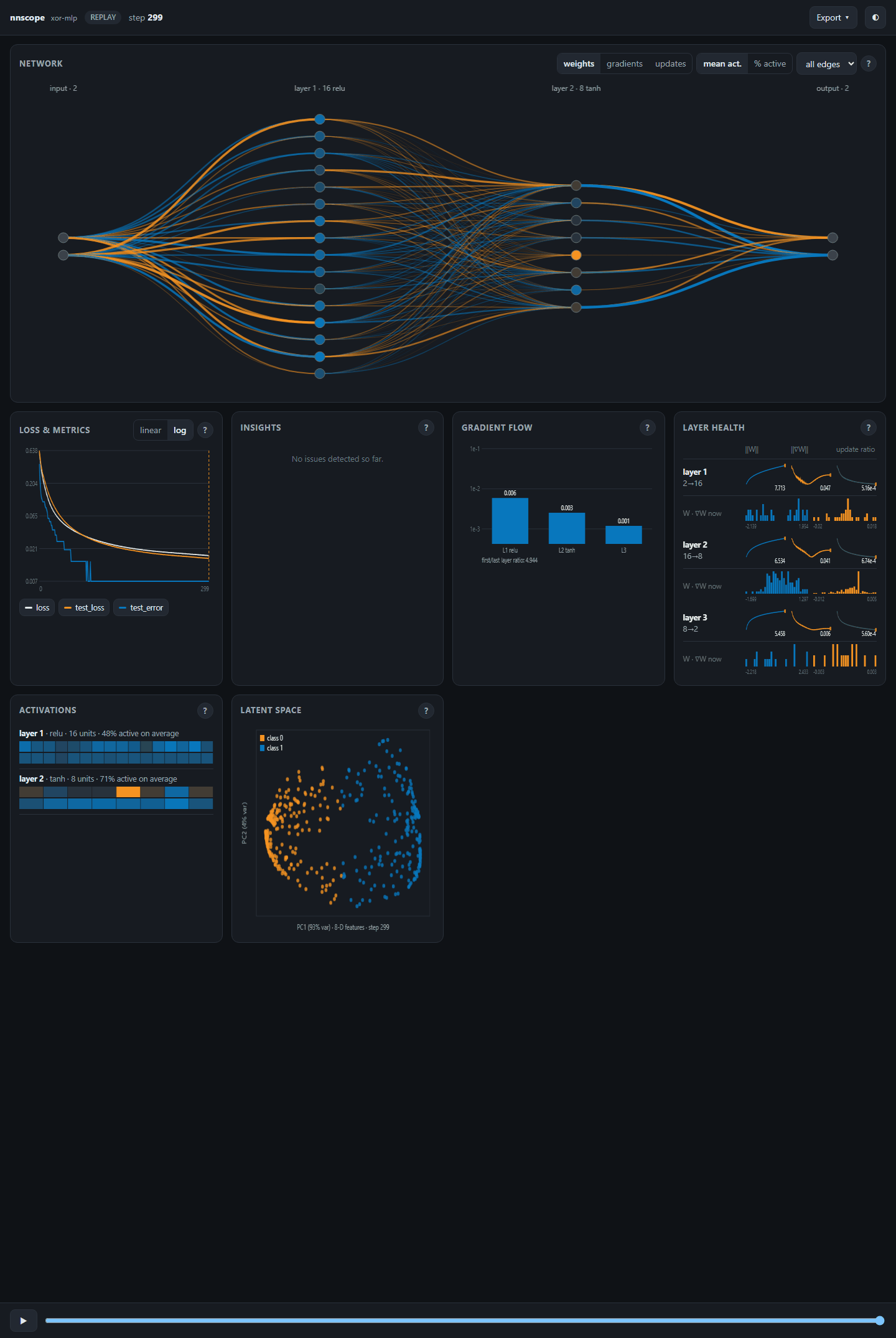
- Zero setup: depends only on NumPy. The dashboard is one self-contained HTML file served by Python's standard library.
- Works with your code: auto-detects common NumPy model layouts, or pass plain arrays.
- Live and replay: a live view while training, then
save_html()for an offline replay with a timeline slider. - Explains itself: every panel has a (?) with the math behind it, and an insights feed diagnoses common problems.
- Responsive: works on a phone (the network turns vertical), light and dark themes.
Install
pip install nnscope            # NumPy is the only dependency
pip install "nnscope[png]"     # optional: PNG snapshots from Python via matplotlib
Quickstart
import nnscope

scope = nnscope.Scope("my-mlp")                    # opens http://127.0.0.1:8765 in your browser
for epoch in range(epochs):
    ...                                             # your own forward pass, backprop and SGD step
    scope.log(epoch, model=model, loss=train_loss, metrics={"test_loss": test_loss})

scope.save_html("run.html")                         # standalone replay, no server needed
scope.snapshot("run.svg")                           # network structure + loss curve as an image
scope.wait()                                        # keep the live page up until Ctrl+C
In a Jupyter notebook, scope.show() puts the live dashboard inline. Use nnscope.Scope(..., live=False) to only record
(for save_html / snapshot).
Connecting your network
nnscope never runs your network; it only reads arrays you already have.
1. A model object (auto-detected). Any object with a .layers list whose dense layers expose weights and biases,
optionally with their gradients:
| what | attribute names tried |
|---|---|
| weights | W, weight, weights, kernel |
| biases | b, bias |
| gradients | dW, grad_W, W_grad, dweight, … and db, grad_b, … |
| cached input (→ activation stats of the previous layer) | x, input, inputs, a_prev |
Layers without weights are recognised as activations by class name (ReLU, Tanh, Sigmoid, LeakyReLU, …), so the graph
shows relu, tanh, … on each layer. CS231n-style parameter dicts ({"W1": …, "b1": …} plus a matching grads dict)
and lists of (W, b) pairs work too.
2. Plain arrays. No model object needed:
scope.log(step, weights=[W1, W2], biases=[b1, b2], grads=[dW1, dW2], loss=loss)
Both x @ W (W is (in, out)) and W @ x (W is (out, in)) conventions are detected from how the shapes chain. Force
one with Scope(layout="in_out") or layout="out_in" if a network is ambiguous (e.g. every layer square).
Optional extras for richer views:
scope.log(step, model=model, loss=loss,
          activations=[a1, a2],     # per-layer outputs on a batch → activation statistics
          deltas=[d1, d2, d3],      # per-layer ∂L/∂z on a batch → shown in the gradient-flow panel
          latent=z, labels=y)       # features of any layer → latent-space scatter
How to read the dashboard
| Panel | What it shows | What to look for |
|---|---|---|
| Network | Neurons (circles) and weights (lines): blue positive, orange negative, thickness ∝ |w|. Toggle the lines to gradients ∂L/∂w or updates Δw, and the node colour to mean activation or % active. | Click a neuron: the inspector shows z = Σ wᵢ aᵢ + b with the real numbers from your batch, its strongest inputs, their gradients and how they changed. Dead ReLUs are ringed in red. |
| Loss & metrics | Every scalar you log over time (log or linear scale). | Spikes: learning rate too high. Test loss rising while training loss falls: overfitting. |
| Insights | Plain-language diagnoses, each at the step where it appeared. Click to jump there. | Vanishing/exploding gradients, dead or saturated units, learning rate too high/low, overfitting. |
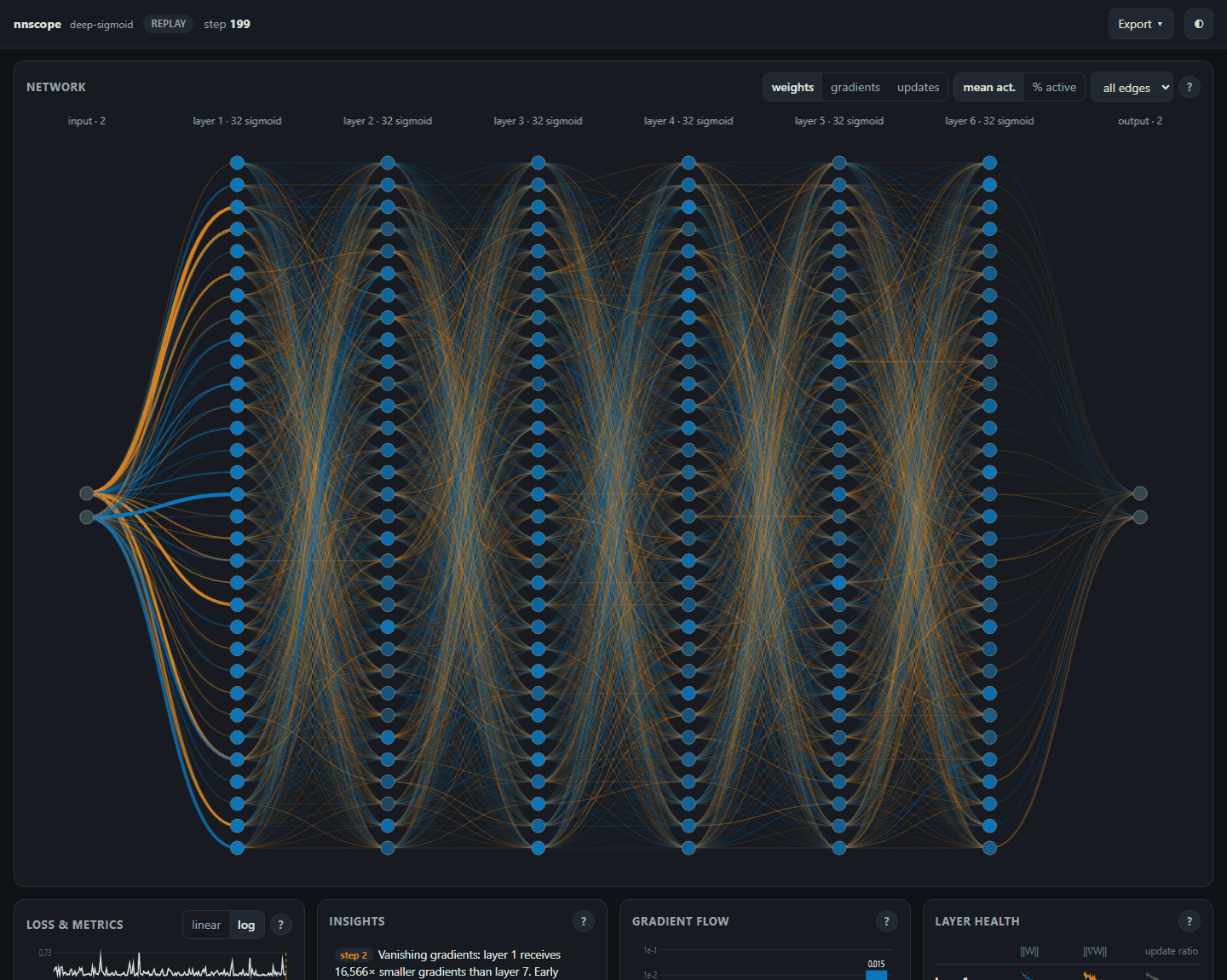
| Gradient flow | Mean |∂L/∂W| per layer, input → output, log scale. | Bars shrinking towards the input = vanishing gradients (e.g. deep sigmoid nets). |
| Layer health | ‖W‖, ‖∇W‖ and the update ratio ‖ΔW‖/‖W‖ per layer over time, plus W and ∇W histograms. | Update ratio ≈ 10⁻³ per SGD step is healthy; ≈ 10⁻¹ is too high. |
| Activations | Per neuron: mean activation and fraction of samples where it is active. | Neurons at 0 % active pass no gradient back and have stopped learning. |
| Latent space | Any layer's features (PCA if wider than 2), coloured by label, along the timeline. | Classes starting mixed and ending linearly separable: the network is building a representation. |
Use the timeline at the bottom (or ← → and space) to replay training. Export saves the network (SVG/PNG), the loss curve, the whole dashboard (PNG) or the raw run data (JSON).
Examples
The examples/ folder uses a tiny homework-style NumPy MLP (_mlp.py). Run them from that folder;
add --no-open to skip opening a browser tab, or --headless to only write runs/*.html and runs/*.svg.
| script | story |
|---|---|
01_quickstart_xor.py |
the basics: an MLP on XOR-like data, live |
02_plain_arrays.py |
no model object: raw W1, b1, W2, b2, hand-written backprop, deltas= |
03_latent_bottleneck.py --k 2 |
watch a k-unit bottleneck layer separate two classes (try --k 32) |
04_vanishing_gradients.py --act sigmoid |
deep sigmoid net: gradients vanish, the insight explains why (compare --act relu) |
05_inr_spectral_bias.py [--fourier] |
fit an image f(x, y) → rgb: raw coordinates plateau, Fourier features keep improving |
API
nnscope.Scope(name="run", *, live=True, port=8765, host="127.0.0.1", open_browser=True, max_neurons=32,
              snapshot_every=None, max_snapshots=300, max_records=5000, layout="auto", latent_points=1000, quiet=False)
log(step=None, *, model=None, loss=None, metrics=None, weights=None, biases=None, grads=None, bias_grads=None, activations=None, deltas=None, latent=None, labels=None, snapshot=None)save_html(path): standalone replay.snapshot(path, step=None):.svg(no dependencies) or.png(matplotlib).show(height=820): Jupyter IFrame.wait(): serve until Ctrl+C.close(); also usable as a context manager.data(): everything recorded so far as a JSON-serialisable dict.
Keeping it light. Scalars are recorded at every log; full snapshots (edges, histograms, latent points) are thinned
adaptively so a run keeps at most max_snapshots of them. Layers wider than max_neurons draw an evenly spaced subset
(statistics always use all neurons). The live stream batches updates to about 10 per second.
Limitations. Dense (fully-connected) layers only for now; convolutional layers are not drawn. The server binds to localhost by default.
Development
uv sync --dev
uv run --dev pytest
License
MIT
1 maintainer

Metadata
1 maintainer
Release files for nnscope 0.1.0
For a detailed explanation of source distributions (sdists) and built distributions (wheels), please see the package formats documentation.
Source distribution (sdist)
| File | Size | Uploaded | |
|---|---|---|---|
| nnscope-0.1.0.tar.gz | 36.9 kB | Details |
Built distribution (wheel)
| File | Interpreter | ABI | Platform | Reset |
|---|---|---|---|---|
| nnscope-0.1.0-py3-none-any.whl | Python 3 | none | any | Details |
Total release size: 77.3 kB
Release files / nnscope-0.1.0.tar.gz
| Download URL | nnscope-0.1.0.tar.gz |
|---|---|
| Size | 36.9 kB |
| Tags | Source |
|
SHA-256 checksum How to use checksums |
90feaca10aeee35461a60c9dcc4b3ce56bc72460296f3bc93c7c32904235f784
|
|
BLAKE2b-256 checksum How to use checksums |
5ade15c5c954fbe5ec682a83c9d14dbff9cede4ec7cff423858ba513f3ed21ba
|
| Upload date | |
|
Uploaded using Trusted Publishing? What is trusted publishing? |
Yes |
| Uploaded via |
twine/7.0.0 CPython/3.13.14
|
Provenance
Provenance describes where a file came from. On PyPI, provenance is shared via attestations, which provide a verifiable record of the build or publishing details. View details, limitations and caveats.


PyPI Publish Attestation
PyPI verified that this artifact, at this checksum, originated from the publisher listed below.
Signed by GitHub Actions, verified by PyPI on Sep 29, 2026.
Transparency logRelease files / nnscope-0.1.0-py3-none-any.whl
| Download URL | nnscope-0.1.0-py3-none-any.whl |
|---|---|
| Size | 40.4 kB |
| Tags | Python 3 |
|
SHA-256 checksum How to use checksums |
5ea9b3907c25cf889bcbb7234c4953acc57f15cb9c6fc4e5166fd579d12fe45b
|
|
BLAKE2b-256 checksum How to use checksums |
46b740bee9a252007941781a05f7a06305d1abf300bc270029d978972eb5f63a
|
| Upload date | |
|
Uploaded using Trusted Publishing? What is trusted publishing? |
Yes |
| Uploaded via |
twine/7.0.0 CPython/3.13.14
|
Provenance
Provenance describes where a file came from. On PyPI, provenance is shared via attestations, which provide a verifiable record of the build or publishing details. View details, limitations and caveats.
PyPI Publish Attestation
PyPI verified that this artifact, at this checksum, originated from the publisher listed below.
Signed by GitHub Actions, verified by PyPI on Sep 29, 2026.
Transparency log













