

Otwin is a Python library used to build Digital Twins of physical equipment from physics, data or both, keep them in step with the machine from live measurements, and forecast with an uncertainty band whose coverage has been measured and a skill score earned out of sample against a reference that is hard to beat.






What otwin is for - Quick Install - Get Started
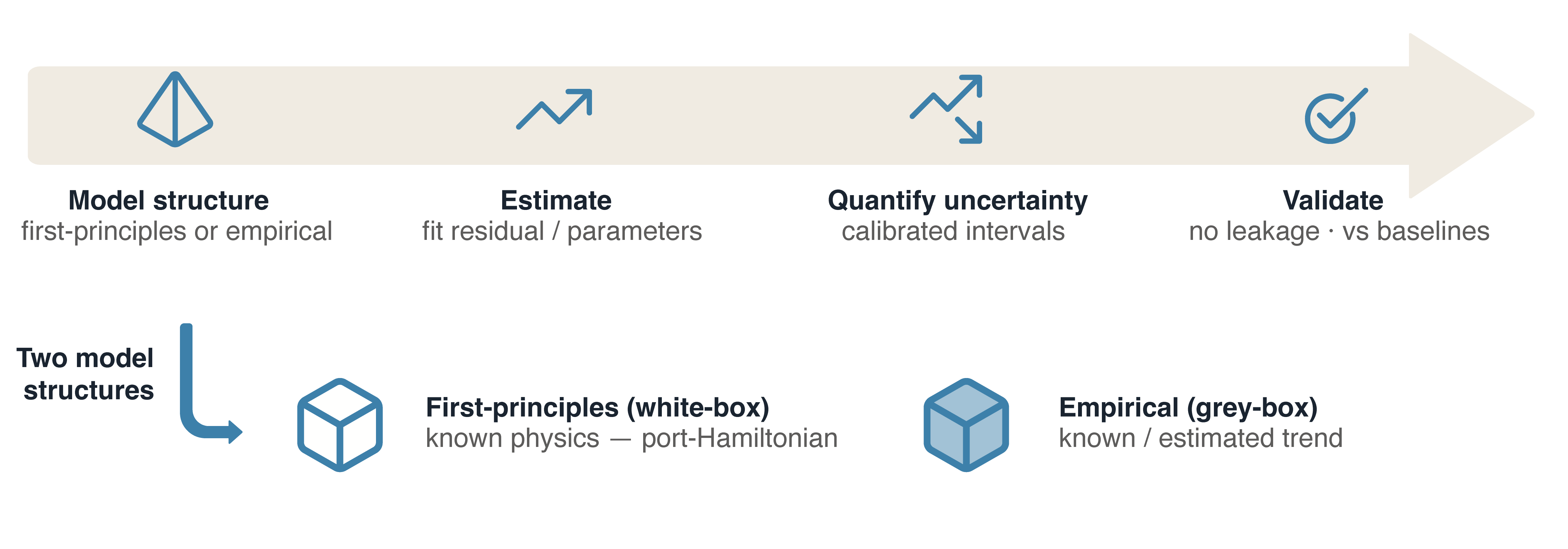
Model - Estimate - Quantify - Validate
Examples - The Otwin project - Issues - Contributing - Citing
What otwin is for
A digital twin is a model of one particular physical asset (machine, pump, battery bank, heat exchanger, chemical reactor, a complete process) kept up to date from that asset's own measurements and run forward to support decissions about it.
Electrical grid. This distribution transformer keeps running above nameplate on hot afternoons. How much longer can it do that before the winding reaches its thermal limit?
Renewable generation and storage. This battery bank is three years into its life. How much can I commit to the market next week and still be certain of delivering it?
Water treatment. The transfer pumps need more power every month for the same flow. How many weeks of margin are left before the duty pump can no longer hold its setpoint?
How much capacity does this Li-ion battery still have? When will it cross the retirement threshold?
What makes otwin different
-
The uncertainty is measured, not declared. A stated 90 % interval means nothing until somebody counts how often it contains the truth.
Interval.is_validatedstaysFalseuntil it has been counted. The conformal example below finishes at a measured 90 % on sixty held-out cycles against a 90 % target; when the calibration set is too small to support the level requested, the library returns an infinite half-width, loudly, rather than a comfortable-looking one. -
The validation is leakage-free and beats something. Partitions are out-of-sample by default, a reference forecaster is mandatory, and the report leads with the skill score against the hardest of persistence, drift, mean and seasonal-naive. The model is handed history and a horizon, never the test values.
-
The twin can say no. Operating range, forecast horizon and calibration status are recorded in the manifest, and a request outside them is refused with a reason rather than answered with a number.
-
A fitted coefficient is not a determined one. A parameter the data cannot pin down is a parameter chosen by the noise, and a forecast that extrapolates through it is extrapolating the noise — while passing every in-window check.
otwin.estimate.identifiabilitytests each coefficient for collinearity, record span and bootstrap stability; the manifest records the verdict; the envelope refuses on it and names the parameter. This is the fourth ground for refusal, and the one that decided every extrapolation result in the study that built this library.
Quick install
pip install otwin
Package-level tree
otwin/
├── io          read equipment or a dataset: SunSpec, Modbus, units, quality      [field]
├── signal      condition the series: resample, find gaps, report coverage
├── model       the physics: port-Hamiltonian, irreversible, catalogue, learned      [nn]
├── estimate    correct the state: EKF, bounded MHE, energy-consistent observer; identifiability
├── forecast    predict and prove it: baselines, skill, conformal, ensembles         [gp]
├── advise      the validated envelope: answer, or refuse with a reason
└── interfaces  the contract the other six compose through — protocols, no algorithms
otwin/interfaces sits outside the chain: the six packages compose through protocols rather than by importing each other, so you can take one on its own — score a model that has nothing to do with otwin, or write physics and never touch io.
Get started
A white-box example consisting of a mass on a spring with a damper. The system has two energy stores: the spring and the moving mass.
import numpy as np
from otwin.model import PortHamiltonianSystem, integrate_phs

# State: x[0] = spring displacement q [m], x[1] = momentum p = m*v [kg m/s]
# k = 2 N/m, m = 1 kg, c = 0.3 N s/m
osc = PortHamiltonianSystem(
    H      = lambda x: 0.5 * 2.0 * x[0]**2 + 0.5 * x[1]**2,   # stored energy [J]
    grad_H = lambda x: np.array([2.0 * x[0], x[1]]),          # [force, velocity]
    J      = lambda x: np.array([[0.0, 1.0], [-1.0, 0.0]]),   # spring <-> mass exchange
    R      = lambda x: np.array([[0.0, 0.0], [0.0, 0.3]]),    # the damper
    g      = lambda x: np.array([[0.0], [1.0]]),              # external force on the mass
    n_states=2, n_inputs=1,
)

t   = np.linspace(0, 20, 400)      # 20 s
u   = np.zeros((400, 1))           # ports closed: no external force
sol = integrate_phs(osc, np.array([1.0, 0.0]), t, u)

E = np.array([osc.energy(x) for x in sol["x"]])
print(f"Stored energy: {E[0]:.4f} J at t=0  ->  {E[-1]:.4f} J at t=20 s")
print(f"Largest single-step energy INCREASE: {max(np.max(np.diff(E)), 0.0):.2e} J")
Stored energy: 1.0000 J at t=0  ->  0.0024 J at t=20 s
Largest single-step energy INCREASE: 0.00e+00 J
That second line Largest single-step energy INCREASE: 0.00e+00 J show that with no force applied, stored energy never rises because the model form makes it impossible.
Model structure
Physical assets like real equipment or complete processess are rarely fully known or fully unknown. Otwin provides five model classes and the manifest records which one you used, because the guarantees available to you depend on the answer.
Digital Twins can be classified as:
 |
White box | Every equation and every parameter comes from first principles. Nothing is fitted. The guarantee is structural — and so is the limit: it can only describe what you can write down. |
 |
Grey box | The structure is fixed by physics; the unknown parts are estimated from data. Almost every useful industrial twin is here. |
 |
Black box | The data decides everything. Excellent inside the range it has seen, and no reason to behave outside it. |
When the physics is known (white-box)
Choose a port-Hamiltonian structure and conservation stops being something you check and becomes something you cannot violate: it is an algebraic property of how the model is written, so it survives any parameter set, any step size and any length of run.
In the first example below, stored energy does not rise on a single step of a 400-step simulation
with the ports closed, where scipy.integrate.solve_ivp on the same right-hand side gains
3.2e-05 J. On the reference cases the same structure reproduces closed-form answers to the limit of
double precision — a pumped-hydro round-trip efficiency agrees with its analytic value to a relative
error of 9.6e-16 — and the irreversible form holds the second law across a full reactor run in
which the same process written as a plain energy balance violates it on 91 % of steps.
What none of this gives you: accuracy. A model with the wrong parameters is still wrong — it is simply wrong without violating the energy balance. Accuracy is measured separately, and that is what the rest of the library is for.
Writing a first-principles model using Port-Hamniltonian Systems (PHS)
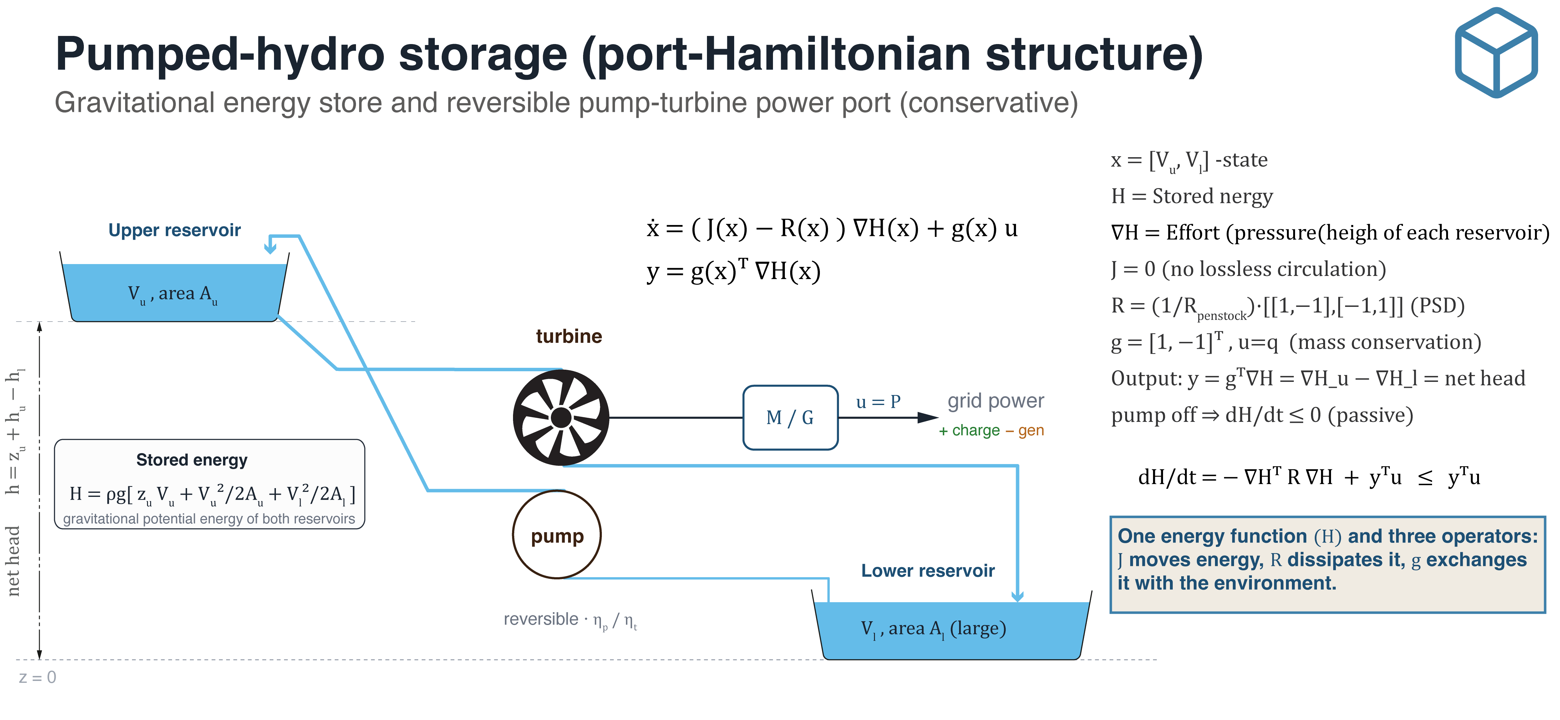
You describe the system with four functions of the state. The dynamics follow from them:
ẋ = dx/dt = ( J(x) - R(x) ) @ grad_H(x)  +  g(x) @ u        # how the state moves (for example how energy changes)
y = g(x).T @ grad_H(x)                                      # what the port delivers
| You write | It means | Water tank example |
|---|---|---|
H(x) |
Total stored energy [J] | 0.5 * rho * g * A * h**2 |
grad_H(x) |
Gradient of that energy — the effort variable: pressure, voltage, force, temperature | Pressure at the base |
J(x) |
Power routed between internal stores, losslessly. Must satisfy J = -J.T |
Zero — only one store |
R(x) |
Dissipation to heat. Must be positive semidefinite | Outlet orifice loss |
g(x) |
The ports — where power crosses the boundary | Inlet pipe |
u is the port input (a flow: m³/s, A, N) and y the port output (an effort: Pa, V, m/s). Their
product y.T @ u is power in watts.
Applications
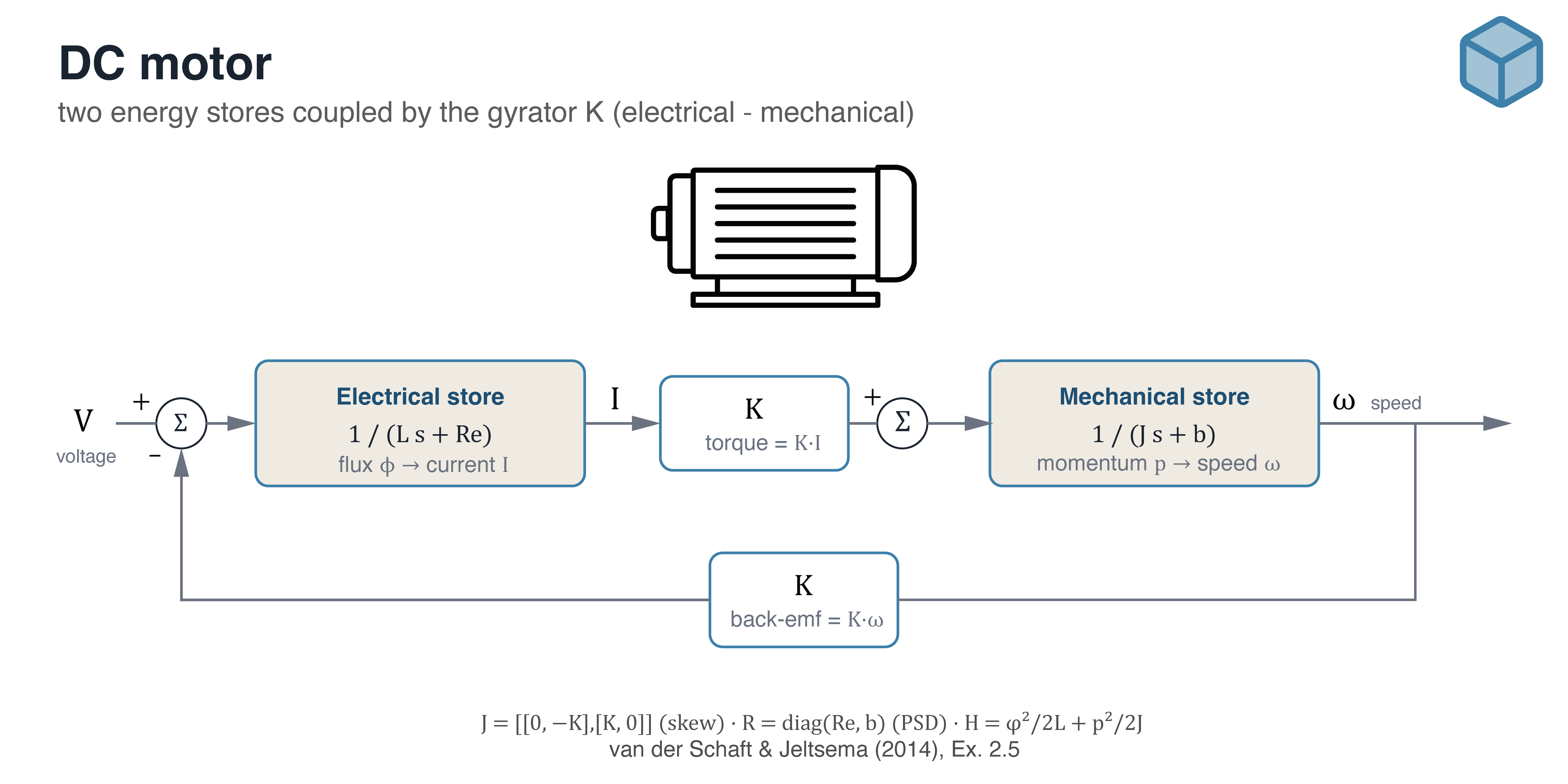
What J, R, H, g already are to you |
|
|---|---|
| Mechanical | A bond graph. J is the junction structure with its transformers and gyrators, R the R-elements, H the C- and I-elements |
| Electrical | An equivalent circuit. grad_H are node voltages and branch currents, J the lossless interconnection, R the resistive network |
| Chemical / process | An energy balance on a control volume, with internal exchange separated from irreversible loss |
| Control | A dissipative system in the sense of Willems. H is the storage function, y.T @ u the supply rate |
The library only asks you to write the four parts down separately instead of collapsing them into a single right-hand side.
A complete model
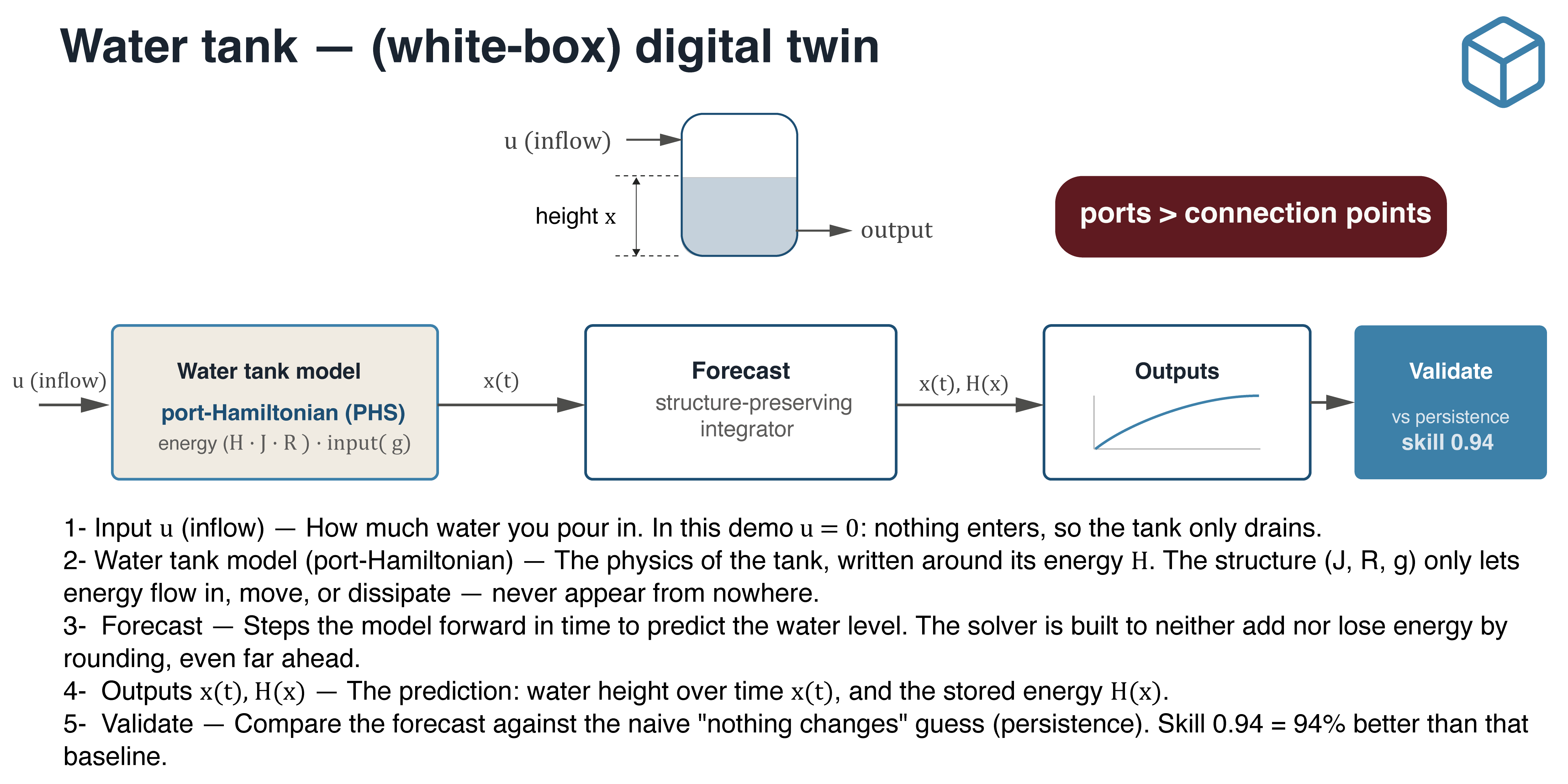
import numpy as np
from otwin.model import PortHamiltonianSystem

A, a, c_d, rho, g_acc = 1.0, 0.1, 0.6, 1000.0, 9.81   # area, orifice, Cd, density, gravity

tank = PortHamiltonianSystem(
    H      = lambda x: 0.5 * rho * g_acc * A * float(x[0])**2,       # energy of the column
    grad_H = lambda x: np.array([rho * g_acc * A * x[0]]),           # pressure at the base [Pa]
    J      = lambda x: np.zeros((1, 1)),                             # one store, nothing circulates
    R      = lambda x: np.array([[c_d * a * np.sqrt(2 * g_acc / max(float(x[0]), 1e-9))
                                  / (rho * g_acc * A**2)]]),         # Torricelli outflow
    g      = lambda x: np.array([[1.0]]),                            # inlet pipe
    n_states=1, n_inputs=1,
)

for name, (ok, margin) in tank.check_structure(np.array([2.0])).items():
    print(f"{name:8s} {'pass' if ok else 'FAIL'}   margin {margin:.3e}")
J_skew   pass   margin 0.000e+00
R_psd    pass   margin 1.916e-05
check_structure is worth running every time you write a model. It catches sign errors and
mis-transposed matrices immediately, before they turn into a plausible-looking wrong answer.
This model ships as otwin.model.water_tank. Also in the library you can find other examples: mass_spring_damper,
dc_motor, pumped_hydro and heat_exchanger.
The port as feedback
A converter holding constant power, a thermostat, a droop-controlled inverter, a level valve — in
all of them u depends on the state. If you pass a callable, the control law is evaluated at the step
midpoint inside the implicit solve, which keeps the discrete power balance intact:
import numpy as np
from otwin.model import water_tank, integrate_phs

tank = water_tank()
t    = np.linspace(0, 600, 601)          # 10 minutes

# Inlet valve on level feedback: u is not a schedule, it is a control law.
res = integrate_phs(tank, np.array([2.0]), t,
                    u=lambda t, x: np.array([max(0.0, 5.0 * (1.5 - float(x[0])))]))

h, q = np.array(res["x"])[:, 0], np.array(res["u"])[:, 0]
print(f"level  {h[0]:.3f} m -> {h[-1]:.3f} m")
print(f"inflow {q[0]:.3f} -> {q[-1]:.3f} m3/s   (outflow at that level: "
      f"{0.6 * 0.1 * np.sqrt(2 * 9.81 * h[-1]):.3f} m3/s)")
level  2.000 m -> 1.436 m
inflow 0.000 -> 0.319 m3/s   (outflow at that level: 0.319 m3/s)
The tank settles below its 1.5 m setpoint, because proportional-only control leaves an offset. res["u"] is what the port actually did. with a governing law there is no schedule to read back.
Processes that produce entropy: Irreversible Port-Hamiltonian Systems (I-PHS)
A chemical reaction, heat conduction, a heat exchanger — any irreversible process needs more than
reversible-plus-dissipative. IrreversiblePHS adds an entropy term to Port Hamiltonian Systems with sigma >= 0 enforced
structurally; IrreversiblePHS.from_modulated(...) gives the Ramírez–Maschke–Sbarbaro form that
most chemical reactor and heat exchanger models fall out. The IrreversiblePHS checked on every
call the second law. otwin.model.heat_exchanger is a worked instance, with effectiveness_ntu for its steady-state check.
Hybrid Digital Twins (grey-box)
This is the most common case we can find. Combine all governing equations can be mathematically tricky and computationally unfeasible. These limitation can be managed with an hybrid approach combining basic governing equations plus observed data.
Hybrid Digital Twins are the most useful models in practice. Keep the analytic model as a prior and learn the residual, so the mean stays physically consistent and the correction carries calibrated uncertainty:
import numpy as np
from otwin.forecast import GPPHS

# The plant has quadratic drag. The analytic model we trust only knows linear damping,
# so the physics is right in structure and wrong in the loss term.
def truth(x, u):
    return np.array([x[1], -2.0*x[0] - 0.9*x[1]*abs(x[1])])

def phs_prior(x, u):
    return np.array([x[1], -2.0*x[0] - 0.3*x[1]])

rng  = np.random.default_rng(0)
X    = rng.uniform(-1.2, 1.2, size=(120, 2))
dXdt = np.array([truth(x, None) for x in X])

np.random.seed(0)   # GPPHS does not yet seed its own hyperparameter restarts
hybrid = GPPHS(n_states=2, prior_dynamics=phs_prior).fit(X, dXdt)

test  = rng.uniform(-1.0, 1.0, size=(40, 2))
exact = np.array([truth(x, None) for x in test])
mean, std = hybrid.predict(test, return_std=True)

err_prior  = np.sqrt(np.mean((np.array([phs_prior(x, None) for x in test]) - exact)**2))
err_hybrid = np.sqrt(np.mean((mean - exact)**2))
far        = hybrid.predict(np.array([[3.0, 3.0]]), return_std=True)[1].mean()

print(f"prior alone   RMSE on dx/dt : {err_prior:.4f}")
print(f"prior + GP    RMSE on dx/dt : {err_hybrid:.4f}")
print(f"GP std inside the fitted range : {std.mean():.4f}")
print(f"GP std far outside it          : {far:.4f}")
prior alone   RMSE on dx/dt : 0.1731
prior + GP    RMSE on dx/dt : 0.0055
GP std inside the fitted range : 0.0056
GP std far outside it          : 0.4593
Thirty times closer on the derivative, and — the part that matters operationally — the predictive standard deviation is two orders of magnitude larger at a state the GP has never seen. The correction knows when it is extrapolating even though the prior does not.
You can find a specific repository for modelling a Li-ion capacity in the repository [https://github.com/otwin-core/otwin-hybrid.git]
Estimating state from measurements
| Estimator | Use it when |
|---|---|
ExtendedKalmanFilter |
The standard case: nonlinear model, Gaussian-ish noise |
MovingHorizonEstimator |
The state has physical bounds. A state of charge is not allowed to be 1.05 |
EnergyConsistentObserver |
The correction itself must respect the energy balance |
The moving-horizon estimator accepts box constraints on the state, and on the reference case it is also 39 % more accurate for it. The energy-consistent observer limits any correction so it cannot increase stored energy beyond what the ports supplied; the trade-off is in the docstring — with ports closed the allowed increase is zero, so a correction that merely reflects an under-energetic prior is rejected too.
Quantifying uncertainty
An interval has meaning if it's coverage has been measured: a stated 90 % interval should contain the truth about 90 % of the time.
import numpy as np
from otwin.forecast import rolling_origin_residuals, horizon_conformal

rng      = np.random.default_rng(0)
cycles   = np.arange(300)
capacity = 1.0 - 2.6e-4*cycles - 4.0e-3*np.sqrt(cycles) + rng.normal(0, 1.5e-3, 300)

class FadeLaw:
    """Fits C = C0 - a*n - b*sqrt(n) to the history, then extrapolates it."""
    def forecast(self, history, horizon):
        h = np.asarray(history, float).ravel()
        n = np.arange(len(h))
        coef, *_ = np.linalg.lstsq(np.column_stack([np.ones_like(n), n, np.sqrt(n)]), h, rcond=None)
        f = np.arange(len(h), len(h) + horizon)
        return (np.column_stack([np.ones_like(f), f, np.sqrt(f)]) @ coef).reshape(-1, 1)

train = capacity[:240]
def refit_forecast(history, horizon):
    return FadeLaw().forecast(history, horizon).ravel()

# Refit at earlier origins and keep genuine h-step-ahead errors -- not in-sample residuals.
residuals, horizons = rolling_origin_residuals(refit_forecast, train, step=5, max_horizon=60)
band = horizon_conformal(residuals, horizons, level=0.90, max_horizon=60)

lower, upper = band.apply(refit_forecast(train, 60))
truth = capacity[240:300]                      # the 60 cycles the band never saw

print(f"{residuals.size} residuals over horizons 1..{horizons.max()}")
print(f"half-width {(upper[0]-lower[0])/2:.4f} at h=1, {(upper[-1]-lower[-1])/2:.4f} at h=60")
print(f"measured coverage: {np.mean((truth >= lower) & (truth <= upper)):.0%}  (target 90%)")
1590 residuals over horizons 1..60
half-width 0.0023 at h=1, 0.0030 at h=60
measured coverage: 90%  (target 90%)
Validation
A model is not validated until its forecasts have been compared, out of sample, against a reference
that is hard to beat. Same series and same FadeLaw as above:
from otwin.forecast import evaluate

print(evaluate(FadeLaw(), capacity.reshape(-1, 1),
               protocol="rolling_origin", n_folds=5, horizon=30))
EvalReport (rolling_origin, 5 folds)
────────────────────────────────────────────────────────────────
Skill Score (vs best baseline): 0.77 (77% better)
Baseline: persistence

Point Metrics:
  RMSE      0.0017 (baseline: 0.0074)
  MAE       0.0014 (baseline: 0.0064)
  NRMSE     0.1141
  MASE      0.8292
  THEIL_U   0.2395
────────────────────────────────────────────────────────────────
Three conventions are built into that one call, because each corrects a mistake that is easy to make and hard to notice:
- Partitions are out-of-sample by default. A random split on a time series trains on Tuesday and
Thursday to predict Wednesday, which measures interpolation.
random_splitexists, warns loudly, and marks the report. - A reference forecaster is required, and the report leads with the skill score. Model error
divided by reference error, against the hardest of persistence, drift, mean and seasonal-naive.
R²is available but never shown first: on a trending series it commonly reads above 0.95 for a model that loses to repeating the last observed value. - The model is given history and a horizon, never the test values. If you supply exogenous
drivers with
exog=, every column is checked against the target first, and the report records that drivers were used — a skill score computed with the future of the drivers in hand is not comparable with one computed without.
Was the parameter determined by the data?
A two-term fade law fits its training window at least as well as a one-term law — it has one more degree of freedom — and reveals the difference only outside the window, as a curve that runs away. By then the manifest says validated and calibrated, because both were measured inside the window. The check that catches it has to run on the fit itself.
identifiability takes the design matrix and the observations and returns one verdict per
coefficient from three tests: collinearity (can this column be reproduced from the others — the
early-life two-term law), span (is the record longer than the fitted time constant — the
asymptotic fouling law), and stability (does a bootstrap over units, not rows, land on the same
value — three field tests per system). Here, the same law on a short and a long window of one cell:
import numpy as np
from otwin.estimate import identifiability

rng = np.random.default_rng(0)
n_all = np.arange(1.0, 801.0)
soh = 1 - 2.0e-3 * n_all**0.5 - 2.0e-9 * n_all**2.5 + rng.normal(0, 1.5e-3, n_all.size)

reports = {}
for window in (100, 800):
    n = n_all[:window]
    X = np.column_stack([n**0.5, n**2.5])                       # the two-term basis
    reports[window] = identifiability(X, 1 - soh[:window], names=("c_slow", "c_knee"),
                                      nonneg=True, n_boot=200)
    print(f"{window} cycles -> {reports[window].verdicts}")
print(reports[100].parameters[1])
100 cycles -> {'c_slow': True, 'c_knee': False}
800 cycles -> {'c_slow': True, 'c_knee': True}
c_knee: NOT identified (collinearity R²=0.758, bootstrap CV=0.72)
    bootstrap over 100 units gives CV=0.72 > 0.5; refitting on a resampled fleet returns a different value
    coefficient switches off or changes sign across bootstrap resamples
Same law, same cell, same code. At 100 cycles the knee coefficient was chosen by the noise; at 800 it was determined by the data. The report also says which test failed: the columns are distinguishable in principle (collinearity 0.76), there is simply not enough knee in the window yet — so the answer is to wait for data, not to change the law. The verdicts go into the manifest below.
Recording where the model is valid
The manifest carries which structure you chose, which parameters were estimated, whether they were identified, how the model was validated and how the band was calibrated. The envelope turns that record into an answer or a refusal.
from otwin.advise import Envelope
from otwin.interfaces import TwinManifest, Provenance

twin = TwinManifest(
    name="cell-A3",
    model_class="empirical_law",          # one of: port_hamiltonian, irreversible_phs,
    model_kind="capacity_fade",           #         empirical_law, learned_phs, composite
    n_states=1, n_inputs=1,
    parameters={"C0": 0.9993, "a": 2.61e-4, "b": 4.02e-3},
    estimated=("C0", "a", "b"),           # three parameters came from data, so: grey box
    provenance=Provenance(created="2026-08-22", otwin_version="0.3.0", seed=0),
    validation=TwinManifest.validated_by("rolling_origin", rmse=0.0017, skill_score=0.77),
    calibration=TwinManifest.calibrated_by("horizon_conformal", empirical_coverage=0.90,
                                           level=0.90, max_horizon=60),
    identification=TwinManifest.identified_by("collinearity+bootstrap",
                                              parameters={"C0": True, "a": True, "b": False}),
)
print("white box?", twin.is_white_box, " validated?", twin.is_validated,
      " identified?", twin.is_identified)

envelope = Envelope(state_bounds=[(0.60, 1.00)], max_horizon=60, requires_identified=True)
print(envelope.check(state=[0.83], horizon=30,  manifest=twin).explain())
white box? False  validated? True  identified? False
outside the validated envelope:
  - identification: extrapolation depends on parameters the data did not determine: b. A fitted
    value the fleet cannot pin down is a value chosen by the noise

This is a refusal, not a failure. The twin has not been shown to answer this question, and
returning a number anyway would hide that.
Inside the operating range, inside the validated horizon, validated and calibrated — and refused, naming the coefficient. With all three parameters identified the same request is answered:
twin_ok = TwinManifest.from_dict({**twin.to_dict(),
    "identification": TwinManifest.identified_by("collinearity+bootstrap",
                                                 parameters={"C0": True, "a": True, "b": True})})
print(envelope.check(state=[0.83], horizon=30,  manifest=twin_ok).explain())
print(envelope.check(state=[0.83], horizon=180, manifest=twin_ok).explain())
inside the validated envelope (horizon 30 <= 60; operating point inside the identified range;
validated, leakage-free; estimated parameters identified)

outside the validated envelope:
  - horizon: beyond the validated forecast horizon (asked for 180, validated to 60)

This is a refusal, not a failure. The twin has not been shown to answer this question, and
returning a number anyway would hide that.
Same discipline as stating the calibration range of an instrument: a reading outside the calibrated
range is reported as such, not returned as a number. is_validated is deliberately strict —
leakage_free must be the boolean True, not merely truthy, because manifests arrive from MATLAB
and Julia where a boolean can round-trip as 1 or as the string "false". is_identified is strict
the same way: every name in estimated must carry the boolean True, and an estimated parameter
with no recorded verdict is not identified — not yet checked is not fine.
Envelope(requires_identified=True) adds the fourth ground for refusal. It is off by default so that
manifests written before 0.4.0 keep working; turn it on for any twin that extrapolates.
Examples
Eight notebook that opens with the question it answers, what otwin does, and what you write yourself; each ends with something to break on purpose. Run them in order the first time. All open in Colab; 01, 02 and 06 need no data file.
| # | notebook | the question | data |
|---|---|---|---|
| 01 | A model that cannot invent energy | How do you know your equations obey physics everywhere, not just where you checked? | simulation |
| 02 | When the process makes entropy | How do you write a reactor model that cannot violate the second law? | simulation |
| 03 | Scoring a forecast so it cannot flatter you | A model forecasts 68 cycles ahead. How good is it, honestly? | NASA PCoE |
| 04 | A band whose 90 % means 90 % | How wide should the interval be, and how do you know? | NASA PCoE |
| 05 | From a noisy sensor to a state you can trust | The sensor says 106 %. What is the state? | NASA PCoE |
| 06 | The twin that says no | What should a twin say when asked something it was never validated for? | simulation |
| 07 | All of it, on eight years of field data | Does the protocol hold on 18 real systems with manual capacity tests as truth? | RWTH field data |
| 08 | Does the physics earn its place? | Would a structured fade law, or a learned residual, narrow that band? | RWTH field data |
Notebooks 03–05 ask for the NASA discharge.csv (upload in Colab). Notebooks 07–08 download
the Source Data spreadsheet of Figgener et al. (2024) from Nature, or accept an upload; without
it they run on a synthetic fleet stamped DEMO. Each notebook's last cell is a regression check —
for CI, not for you.
The otwin project
| Repository | What it is |
|---|---|
| otwin | The library. Start here |
| otwin-spec | The specification and its conformance suite — reference cases with closed-form answers, used to verify that any implementation is correct, in any language |
| otwin-hybrid | A worked case in Python, Julia and R: predicting end of life of a lithium-ion cell from the first 40 % of its life. Opens in Colab in one click |
| otwin-systems | The growing catalogue of physical models, each shipped with a closed-form result it must reproduce |
Julia and MATLAB implementations are open for contributors — otwin-spec tests over a subprocess
interface, so a second-language implementation has an objective completion criterion: pass the suite
unmodified. See CONTRIBUTING.md for that and for a list of self-contained project
topics.
Issues
Contributing
CONTRIBUTING.md. The catalogue of physical models is the easiest place to start, and each contribution is a system you already know plus one closed-form result it must reproduce
Citing
Each repository in otwin prokect include a CITATION.cff
References
- van der Schaft, A. & Jeltsema, D. (2014). Port-Hamiltonian Systems Theory: An Introductory Overview. Foundations and Trends in Systems and Control.
- Willems, J. C. (1972). Dissipative dynamical systems. Arch. Rational Mech. Anal. 45(5).
- Karnopp, D., Margolis, D. & Rosenberg, R. System Dynamics: Modeling, Simulation, and Control of Mechatronic Systems. Wiley.
- Ramírez, H., Maschke, B. & Sbarbaro, D. (2013). Irreversible port-Hamiltonian systems. Chemical Engineering Science 89.
- Greydanus, S., Dzamba, M. & Yosinski, J. (2019). Hamiltonian Neural Networks. NeurIPS 32.
- Rasmussen, C. E. & Williams, C. K. I. (2006). Gaussian Processes for Machine Learning. MIT Press.
- Vovk, V., Gammerman, A. & Shafer, G. (2005). Algorithmic Learning in a Random World. Springer.
- Gneiting, T. & Raftery, A. E. (2007). Strictly proper scoring rules, prediction, and estimation. JASA 102(477).
- ISO 13374 — Condition monitoring and diagnostics of machines.
- ISO 13381-1:2015 — Condition monitoring and diagnostics of machines: prognostics.
1 maintainer

Metadata
1 maintainer
Release files for otwin 0.4.0
For a detailed explanation of source distributions (sdists) and built distributions (wheels), please see the package formats documentation.
Source distribution (sdist)
| File | Size | Uploaded | |
|---|---|---|---|
| otwin-0.4.0.tar.gz | 1.1 MB | Details |
Built distribution (wheel)
| File | Interpreter | ABI | Platform | Reset |
|---|---|---|---|---|
| otwin-0.4.0-py3-none-any.whl | Python 3 | none | any | Details |
Total release size: 1.2 MB
Release files / otwin-0.4.0.tar.gz
| Download URL | otwin-0.4.0.tar.gz |
|---|---|
| Size | 1.1 MB |
| Tags | Source |
|
SHA-256 checksum How to use checksums |
add1311d9210f769ecc6e423157bbc5b1ef169b47a09ea7532c289d2e4f0f3ed
|
|
BLAKE2b-256 checksum How to use checksums |
a64b47f45bc828676a830681fb4ca4e641dfbd9d35ab9e318113489c9858646b
|
| Upload date | |
|
Uploaded using Trusted Publishing? What is trusted publishing? |
Yes |
| Uploaded via |
twine/7.0.0 CPython/3.13.14
|
Provenance
Provenance describes where a file came from. On PyPI, provenance is shared via attestations, which provide a verifiable record of the build or publishing details. View details, limitations and caveats.


PyPI Publish Attestation
PyPI verified that this artifact, at this checksum, originated from the publisher listed below.
Signed by GitHub Actions, verified by PyPI on Aug 25, 2026.
Transparency logRelease files / otwin-0.4.0-py3-none-any.whl
| Download URL | otwin-0.4.0-py3-none-any.whl |
|---|---|
| Size | 188.4 kB |
| Tags | Python 3 |
|
SHA-256 checksum How to use checksums |
8f6a7a9921e5c633781505d0afd4d459f3755b3e830e8d8b3713dba3d043deae
|
|
BLAKE2b-256 checksum How to use checksums |
216fe5b83c08c2b20909e9d4048fc07e5a8ad7c2efb268bd120ee511059f1e95
|
| Upload date | |
|
Uploaded using Trusted Publishing? What is trusted publishing? |
Yes |
| Uploaded via |
twine/7.0.0 CPython/3.13.14
|
Provenance
Provenance describes where a file came from. On PyPI, provenance is shared via attestations, which provide a verifiable record of the build or publishing details. View details, limitations and caveats.
PyPI Publish Attestation
PyPI verified that this artifact, at this checksum, originated from the publisher listed below.
Signed by GitHub Actions, verified by PyPI on Aug 25, 2026.
Transparency log













